Freescale Semiconductor
Application Note
Document Number: AN4247
Rev. 2, 07/2011
Layout Recommendations for PCBs
Using a Magnetometer Sensor
by: Talat Ozyagcilar
Applications Engineer
Introduction
1
This application note is intended to guide engineers in
the successful design of Printed Circuit Boards (PCBs)
incorporating magnetometer sensors. For convenience,
the application discussed is an electronic compass
(or eCompass) designed into a smartphone but the
guidelines are equally applicable to other products using
a magnetometer.
This note covers:
• Characteristics of the geomagnetic field
•
Sensing range and resolution required in the
magnetometer
Contents
1
Introduction . . . . . . . . . . . . . . . . . . . . . . . . . . . . . . . . . . . 1
1.1 Key Words . . . . . . . . . . . . . . . . . . . . . . . . . . . . . . . . 2
1.2 Summary . . . . . . . . . . . . . . . . . . . . . . . . . . . . . . . . . 2
The Geomagnetic Field . . . . . . . . . . . . . . . . . . . . . . . . . . 3
Magnetic Interference within the Smartphone . . . . . . . . . 3
Hard Iron Interference . . . . . . . . . . . . . . . . . . . . . . . . . . . 4
Soft Iron Interference. . . . . . . . . . . . . . . . . . . . . . . . . . . . 5
Fields from PCB Currents . . . . . . . . . . . . . . . . . . . . . . . . 6
Other Sources of PCB Interference. . . . . . . . . . . . . . . . . 7
Component and Material Selection . . . . . . . . . . . . . . . . . 8
Experimental Determination of the Magnetometer
Measurement Locus . . . . . . . . . . . . . . . . . . . . . . . . . . . . 9
10 Mathematical Annex . . . . . . . . . . . . . . . . . . . . . . . . . . . 12
2
3
4
5
6
7
8
9
• Level of accuracy needed from the calibration
software
Physics of magnetic interference from hard and
soft iron effects and PCB currents
•
• Guidelines for component selection
• Experimental approach to visualize field
distortions prior to layout and fabrication of the
PCB
© Freescale Semiconductor, Inc., 2011. All rights reserved.
�
Introduction
The mathematical formalism of hard and soft iron interference is provided in the Mathematical Annex for
engineers wishing to understand the theoretical derivation of ellipsoidal measurement loci.
Additional information on the mathematics of a tilt-compensated eCompass can be found in the Freescale
Application Note AN4248 “Implementing a Tilt-Compensated eCompass using Accelerometer and
Magnetometer Sensors”. This and other application notes can be downloaded from
http://www.freescale.com.
Key Words
1.1
eCompass, Geomagnetic, Magnetometer, Hard Iron, Soft Iron, Layout, Calibration, Ferromagnetic.
1.2
Summary
• A smartphone magnetometer measures the sum of the geomagnetic field plus magnetic
interference generated by ferromagnetic components on the smartphone PCB. This interference is
classified into permanent hard iron and induced soft iron components.
• The magnitude of hard iron and soft iron interference can exceed 1000 μT and saturate the
magnetometer if care is not taken to minimize the use of ferromagnetic components, such as
speakers, and to optimize the PCB layout by placing the magnetometer away from sources of
magnetic interference.
Software calibration algorithms are required to calculate the characteristics of, and mathematically
remove, both hard iron and soft iron interference from the magnetometer readings allowing the
geomagnetic field component to be measured with an error below 0.5 μT.
•
• An experimental approach is described which uses a Freescale RD4247MAG3110 eCompass
evaluation board to measure and visualize the level of hard iron and soft iron interference prior to
PCB fabrication.
Layout Recommendations for PCBs Using a Magnetometer Sensor, Rev. 2
2
Freescale Semiconductor
�
The Geomagnetic Field
The Geomagnetic Field
2
The magnitude of the earth's magnetic field (the geomagnetic field) varies over the surface of the earth
from a minimum of 22 μT over South America to a maximum of 67 μT south of Australia. The heading
of an eCompass is determined from the relative strengths of the two horizontal geomagnetic field
components and these vary from zero at the magnetic poles to a maximum of 42 μT over East Asia.
Detailed geomagnetic field maps are available from the World Data Center for Geomagnetism at
http://wdc.kugi.kyoto-u.ac.jp/igrf/.
A rough and ready estimate of the error in an eCompass heading is given in radians by the ratio of the error
in geomagnetic field estimation to the horizontal geomagnetic field strength. For example, the lowest value
of the horizontal field strength likely to be experienced by a smartphone user is 10 μT in northern Canada
and Russia. A compass heading accuracy of 0.05 radians or 3 degrees therefore requires that the error in
estimating the geomagnetic field be no more than 0.5 μT.
Magnetic Interference within the Smartphone
3
Unlike accelerometer, pressure, and gyroscope MEMS sensors, which use mechanical sensing elements
unaffected by electromagnetic components on the PCB, magnetometers are sensitive to the magnetic fields
generated by other circuit components.
The most common magnetic field sources are:
•
•
•
permanent ferromagnets (as found in speakers or buzzers).
induced fields within any ferromagnetic material lacking a permanent field (such as sheet steel).
fields generated by current flows (ranging from strong currents in power supply tracks to smaller
currents within coils).
Even in a well-designed smartphone, these sources create extraneous fields with magnitudes approaching
1000 μT in the vicinity of the magnetometer placing severe constraints on the performance of both the
magnetometer and the calibration software running within the smartphone eCompass application. The
magnetometer must have an operating range of ±1000 μT to accommodate the sum of the geomagnetic
and interfering fields and the calibration software must identify and remove this interference to accuracy
better than 0.5 μT or one part in two thousand for 1000 μT interference.
Designers should not assume that the calibration software will always correct for a poor layout.
Component selection and layout should therefore be optimized to reduce the interfering fields as much as
is realistically feasible. Smaller interference fields ease the job of the calibration software and result in
more accurate compass headings.
Layout Recommendations for PCBs Using a Magnetometer Sensor, Rev. 2
Freescale Semiconductor
3
�
Hard Iron Interference
Hard Iron Interference
4
'Hard iron' magnetic fields are those which are generated by permanently magnetized ferromagnetic
components on the PCB, such as an audio speaker or buzzer. Permanently magnetized components also
create induced magnetic fields in normally unmagnetized ferromagnetic materials in their vicinity. Since
the magnetometer and all components on the PCB are in fixed positions with respect to each other, the hard
iron interference manifests as an additive magnetic field vector when measured in the magnetometer
reference frame.
It makes little sense for manufacturers to supply carefully calibrated zero field offset magnetometers into
the smartphone market since the magnetometer will be exposed to an unknown additive hard iron field.
The manufacturer will typically specify only the limits between which the zero field offset will lie. The
magnetometer zero field offset is also independent of the smartphone orientation and therefore simply adds
to the hard iron field. The calibration algorithm then adds the magnetometer zero field offset to the PCB
hard iron interference and removes both.
Figure 1 shows the modelling of the distortion of the geomagnetic field by three permanent magnets
creating hard iron interference. The first image shows the field of the permanent magnets in the absence
of an external field. The second image shows the combined field of the permanent magnets and the
external field.
A magnetometer located in the vicinity of the magnets will see the sum of the geomagnetic field and the
hard iron field and will compute an erroneous compass heading in the absence of calibration software.
Figure 1. Hard iron disturbance of a uniform magnetic field
Hard iron interference can be minimized by a common sense strategy of avoiding, or selecting alternatives
to, strongly magnetized ferromagnetic components and placing the magnetometer as far away as possible
from such components.
Layout Recommendations for PCBs Using a Magnetometer Sensor, Rev. 2
4
Freescale Semiconductor
�
Soft Iron Interference
Soft Iron Interference
5
'Soft iron' interference is created by the induction of a temporary magnetic field into normally
unmagnetized ferromagnetic components, such as steel shields and batteries, on the PCB by the
geomagnetic field.
Soft iron effects are more complex to model than hard iron since the induced field depends on the relative
orientation of the geomagnetic field to the soft iron components. Earth's geomagnetic field is a fixed
vector, however, its directional influence on the soft iron field varies and is dependent on the smartphone
orientation. Soft iron effects induced by the geomagnetic field are therefore dependent on the smartphone
orientation.
While the hard iron interfering field can be modelled as a simple additive three-component magnetic field
vector, the soft iron interfering field manifests as axes with high magnetic permeability within the
smartphone and is normally modelled as a six-component symmetric matrix.
Figure 2 illustrates the distortion of a uniform external magnetic field by three unmagnetized
ferromagnetic bars oriented in different directions. The first image shows that there is no field in the
absence of the external field. The second image shows the sum of the induced field in the bars and the
external field. The bars become magnetized by the external field and steer it along their axes.
As shown in the hard iron field example, a magnetometer located in the midst of soft iron components will
measure a magnetic field which may point in a very different direction to the geomagnetic field.
Figure 2. Soft iron disturbance of a uniform magnetic field
Layout Recommendations for PCBs Using a Magnetometer Sensor, Rev. 2
Freescale Semiconductor
5
�
Fields from PCB Currents
Fields from PCB Currents
6
Fixed currents, whether in PCB tracks or within coils, will generate fixed magnetic fields which add to the
hard iron component. Calibration software will attempt to calibrate these fields and remove them, but it is
good practice to minimize these fields. The strength of the resulting field measured at the magnetometer
follows the standard rules of electromagnetism: the generated field is proportional to the current, is
multiplied by coherent addition of the same current in a coil, and reduces with distance from the current
source.
Designers should therefore place high current tracks and coils as far away as possible from the
magnetometer. Ferromagnetic cores within coils become magnetized by both the coil current and the
geomagnetic field creating additional soft iron interference.
An estimate of the magnetic field sourced by a PCB power supply track can be obtained from MAG3110's
equation relating the curl of the magnetic field B to the local current density j and the time derivative of
the local electric field E:
×
∇ B μ0j
=
ε0+
μ0
∂E
-------
∂t
μ0 is the permeability of free space and is defined to have value:
μ0
=
4π 10 7–
×
NA 2–
Eqn. 1
Eqn. 2
If the PCB trace is straight with extent in both directions greater than the separation of the magnetometer
from the trace, then edge effects can be ignored and the magnetic field will be rotationally symmetrical.
With the additional constraint that the electric and magnetic fields are constant, Equation 1 can be
rewritten using Stokes' theorem in terms of line and surface integrals for a closed circular path at normal
distance r0 from the trace:
∫°
B.dr
r
=
2πr0B r0(
)
∇ B×(
).dS
∫∫=
s
μ0 j.dS
∫∫=
s
Eqn. 3
The current density j includes both free currents in the trace and bound currents in ferromagnetic materials.
If there are no ferromagnetic materials in the vicinity of the magnetometer and PCB trace then the surface
integral of the current density j simply equals the PCB trace current I. The return current flow through the
ground plane is assumed to be spatially diffused and is ignored.
Layout Recommendations for PCBs Using a Magnetometer Sensor, Rev. 2
6
Freescale Semiconductor
�
Other Sources of PCB Interference
If, in addition, the less than one part in 106 difference in the magnetic permeability of air and vacuum is
ignored in Equation 3, then the magnetic field B(r0) at distance r0 from the PCB trace is given in Teslas by:
B r0(
)
=
μ0I
-----------
2πr0
=
10 6– I
×
0.2
--------------------------
r0
Eqn. 4
Modern smartphone power traces can easily source 1A in current. At 10-3m separation, the magnetic field
from a 1A current trace will be 200 μT reducing to 20 μT at 10-2m separation. This field will in turn induce
a soft iron field in local ferromagnetic components on the PCB which may amplify the prediction of
Equation 4 several times over.
The effects of time varying currents depend on their frequency. The highest sampling rate of a consumer
magnetometer is approximately 100 Hz so currents at significantly higher frequencies will not be
detectable by the magnetometer. Signals at lower frequencies may be detectable as modulation of the
magnetic output and the compass heading. Incremental changes in current will create corresponding
changes in the magnetic field and compass error.
The most difficult situation for the calibration software is the placement too close to the magnetometer of
a power supply trace supplying a varying current depending on the smartphone processor load, the state
of the LCD backlight and whether the RF power amplifier is active.
Other Sources of PCB Interference
7
PCB designers should also make industrial designers and mechanical engineers aware of the consequences
of including magnetic materials into the smartphone housing. These should generally be avoided since
they add to the overall hard and soft iron field. Industrial designers should be aware that different phone
configurations (such as a clamshell phone being open or closed) also create different magnetic interference
which further complicates the task of the calibration software.
NOTE:
Engineers should not attempt to shield the magnetometer from PCB hard
iron or soft iron interference by placing the magnetometer or the interfering
magnetic materials under shielding. Aluminum shielding is transparent to
magnetic fields and has no effect. Steel shielding acts as an additional source
of soft iron interference distorting both the direction and magnitude of the
geomagnetic field and amplifying the effects of permanently magnetized
components on the PCB.
Layout Recommendations for PCBs Using a Magnetometer Sensor, Rev. 2
Freescale Semiconductor
7
�
Component and Material Selection
Component and Material Selection
8
Components using iron, cobalt, nickel and their alloys (generally referred to as ferromagnets) can maintain
a permanent magnetic field and are the predominant source of hard iron interference. Typical components
with permanent magnetization include speaker magnets, vibrator and camera modules.
The same ferromagnetic materials when normally unmagnetized are responsible for the soft iron magnetic
interference. Any external field, whether the hard iron or the geomagnetic field, induces a temporary
magnetic field in these materials. Common sources of soft iron distortion include the smartphone battery
and steel shields in the RF module.
Materials that are safe for use in the proximity of the magnetometer include brass, aluminum, copper, gold,
silver and titanium.
The ability of a material to develop an induced soft iron field in response to an external field is proportional
to its relative magnetic permeability μr. The relative permeabilities of common materials are shown in
Table 1. Those with high relative permeabilities should be avoided wherever possible.
Table 1. Common Materials
Material
Relative Permeability μr
Mu-metal (75% Ni, 15% Fe, Cu, Mb)
25,000 and higher
Permalloy (80% Ni, 20% Fe)
Iron (99.8% pure)
Ferrite N41
Ferrite M33
Nickel (99% pure)
Cobalt (99% pure)
Steel
Ferrite U60
Platinum
Titanium
Aluminum
Brass
Copper
Silver
Gold
8000
5000
3000
750
600
250
100
8
1.000265
1.00005
1.000022
≈1.00000
0.999994
0.999974
0.99996
Layout Recommendations for PCBs Using a Magnetometer Sensor, Rev. 2
8
Freescale Semiconductor
�

.pdf-第1页.jpg")
.pdf-第2页.jpg")
.pdf-第3页.jpg")
.pdf-第4页.jpg")
.pdf-第5页.jpg")
.pdf-第6页.jpg")
.pdf-第7页.jpg")
.pdf-第8页.jpg")
 V2版本原理图(Capacitive-Fingerprint-Reader-Schematic_V2).pdf
 摄像头工作原理.doc
 VL53L0X简要说明(En.FLVL53L00216).pdf
 原理图(DVK720-Schematic).pdf
 原理图(Pico-Clock-Green-Schdoc).pdf
 原理图(RS485-CAN-HAT-B-schematic).pdf
 File:SIM7500_SIM7600_SIM7800 Series_SSL_Application Note_V2.00.pdf
 ADS1263(Ads1262).pdf
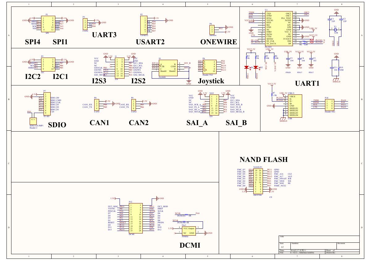 原理图(Open429Z-D-Schematic).pdf
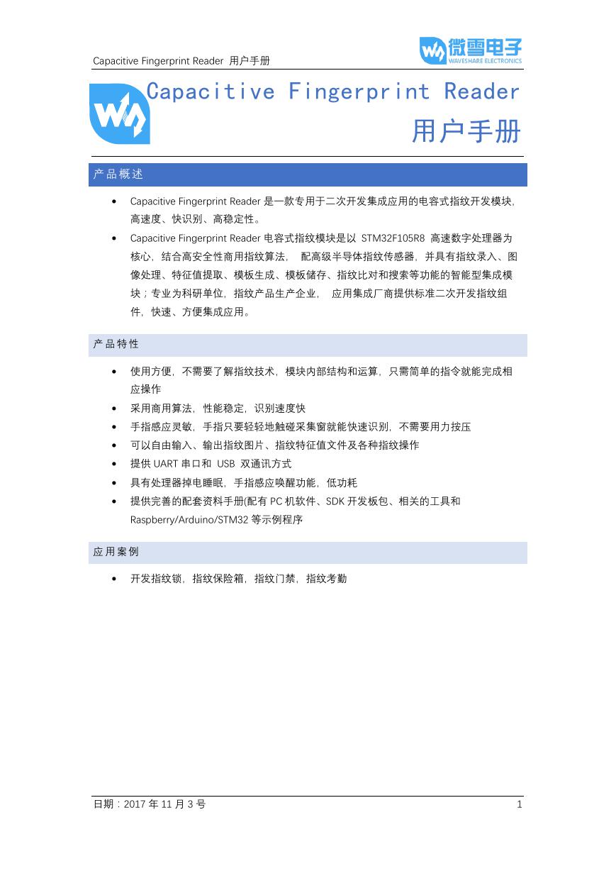 用户手册(Capacitive_Fingerprint_Reader_User_Manual_CN).pdf
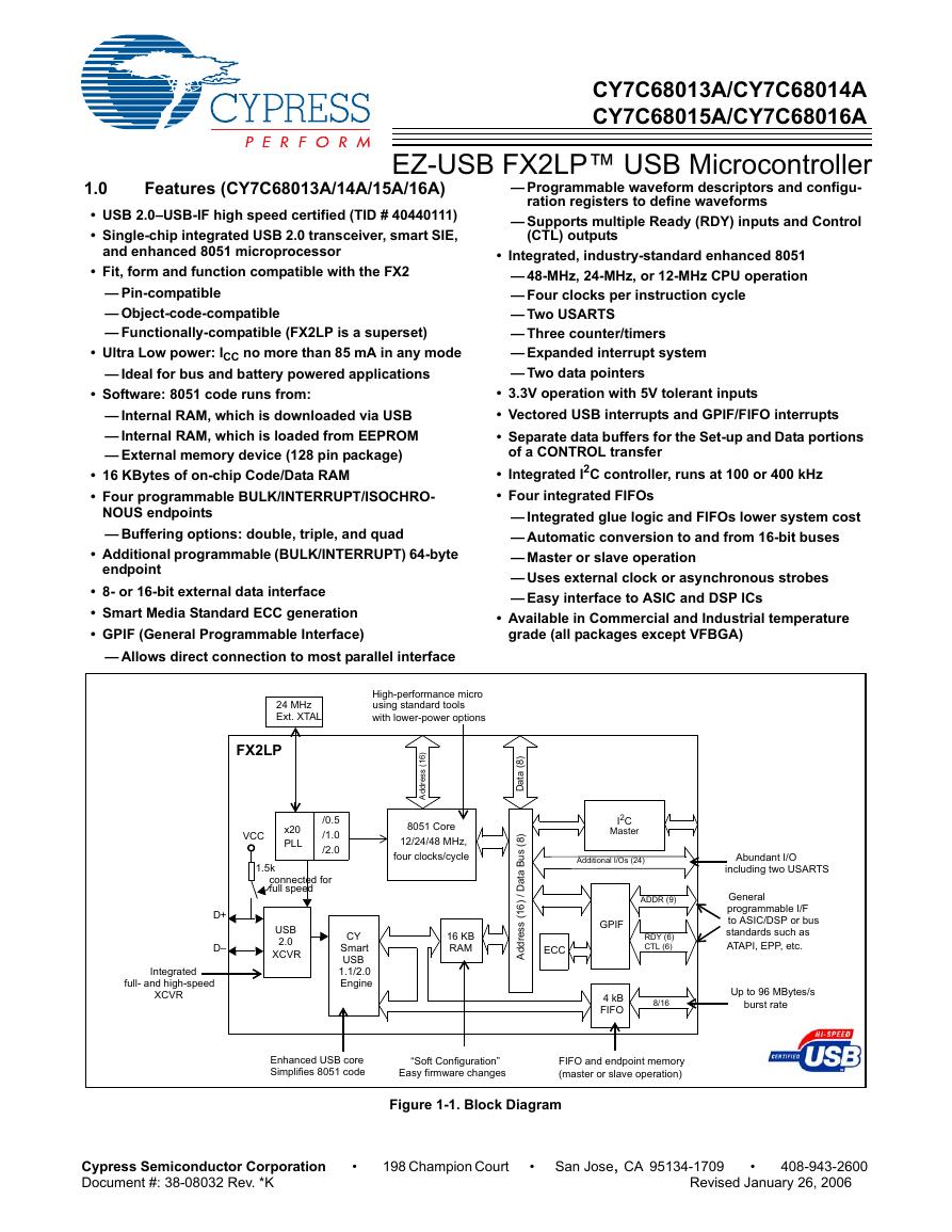 CY7C68013A(英文版)(CY7C68013A).pdf
 TechnicalReference_Dem.pdf
 23-S4P+与IRC5P的差别-ABB喷涂机器人培训.pdf