Freescale Semiconductor
Application Note
Document Number: AN4248
Rev. 0, 03/2011
Implementing a Tilt-Compensated
eCompass using Accelerometer and
Magnetometer Sensors
by: Talat Ozyagcilar
Applications Engineer
Contents
1
2
3
4
5
6
Introduction . . . . . . . . . . . . . . . . . . . . . . . . . . . . . . . . . . . 1
1.1 Key Words . . . . . . . . . . . . . . . . . . . . . . . . . . . . . . . . 2
1.2 Summary . . . . . . . . . . . . . . . . . . . . . . . . . . . . . . . . . 2
Coordinate System and Package Alignment . . . . . . . . . . 3
Accelerometer and Magnetometer Outputs as a Function of
Phone Orientation . . . . . . . . . . . . . . . . . . . . . . . . . . . . . . 4
Tilt-Compensation Algorithm . . . . . . . . . . . . . . . . . . . . . . 6
Estimation of the Hard Iron Offset V . . . . . . . . . . . . . . . . 8
Software Implementation. . . . . . . . . . . . . . . . . . . . . . . . . 8
6.1
eCompass C# Source Code . . . . . . . . . . . . . . . . . . 9
6.2 Modulo Arithmetic Low Pass Filter for Angles C#
Source Code . . . . . . . . . . . . . . . . . . . . . . . . . . . . . 10
6.3 Sine and Cosine Calculation C# Source Code . . . 11
6.4 ATAN2 Calculation C# Source Code. . . . . . . . . . . 13
6.5 ATAN Calculation C# Source Code. . . . . . . . . . . . 14
6.6
Integer Division C# Source Code . . . . . . . . . . . . . 15
Introduction
1
This technical note provides the mathematics, reference
source code and guidance for engineers implementing a
tilt-compensated electronic compass (eCompass).
The eCompass uses a three axis accelerometer and three
axis magnetometer. The accelerometer measures the
components of the earth's gravity and the magnetometer
measures the components of earth's magnetic field (the
geomagnetic field). Since both the accelerometer and
magnetometer are fixed on the Printed Circuit Board
(PCB), their readings change according to the orientation
of the PCB.
If the PCB remains flat, then the compass heading could
be computed from the arctangent of the ratio of the two
horizontal magnetic field components. Since, in general,
the PCB will have an arbitrary orientation, the compass
heading is a function of all three accelerometer readings
and all three magnetometer readings.
© Freescale Semiconductor, Inc., 2011. All rights reserved.
�
Introduction
The tilt-compensated eCompass algorithm actually calculates all three angles (pitch, roll, and yaw or
compass heading) that define the PCB orientation. The eCompass algorithms can therefore also be used to
create a 3-D Pointer with the pointing direction defined by the yaw and pitch angles.
The accuracy of an eCompass is highly dependent on the calculation and subtraction in software of stray
magnetic fields both within, and in the vicinity of, the magnetometer on the PCB. By convention, these
fields are divided into those that are fixed (termed Hard Iron effects) and those that are induced by the
geomagnetic field (termed Soft Iron effects). Any zero field offset in the magnetometer is normally
included with the PCB’s Hard Iron effects and is calibrated at the same time.
This document describes a simple three-element model to compensate for Hard Iron effects. This three-
element model should suffice for many situations. Please contact your Freescale sales representative for
details of a full nine-element model which compensates for both Hard and Soft Iron effects.
The C# language source code listed within this document contains cross-references to the equations used.
These listings contain all the code needed to return the yaw, pitch and roll angles from the magnetometer
and accelerometer sensor readings.
For convenience, the remainder of the this document assumes that the eCompass will be implemented
within a mobile phone.
Key Words
1.1
Accelerometer, Magnetometer, Tilt angles, eCompass, 3-D Pointer, Tilt Compensation, Tilt Correction,
Hard Iron, Soft Iron, Geomagnetism
1.2
Summary
1. A tilt-compensated electronic compass (eCompass) is implemented using the combination of a
three-axis accelerometer and a three-axis magnetometer.
2. The accelerometer readings provide pitch and roll angle information which is used to correct the
magnetometer data. This allows for accurate calculation of the yaw or compass heading when the
eCompass is not held flat.
3. The pitch and roll angles are computed on the assumption that the accelerometer readings result
entirely from the eCompass orientation in the earth's gravitational field. The tilt-compensated
eCompass will not operate under freefall or low g conditions at one extreme nor high-g
accelerations at the other.
4. A 3-D Pointer can be implemented using the yaw (compass heading) and pitch angles from the
eCompass algorithms.
5. The magnetometer readings must be corrected for Hard Iron and Soft Iron effects.
6. A simple three parameter Hard Iron correction algorithm is described. Please contact your
Freescale sales representative for details of Freescale's complete nine parameter Hard and Soft Iron
correction algorithms.
7. Reference C# code is provided at the end of this document for the full tilt-compensated e-Compass
with Hard Iron compensation.
8. Demonstration eCompass platforms are available that show Freescale's latest sensors. Please
contact your Freescale sales representative for details.
2
Freescale Semiconductor
AN4248, Rev. 0
�
Coordinate System and Package Alignment
2
This application note uses the industry standard “NED” (North, East, Down) coordinate system to label
axes on the mobile phone. The x-axis of the phone is the eCompass pointing direction, the y-axis points to
the right and the z-axis points downward. (see Figure 1).
Coordinate System and Package Alignment
Figure 1. Coordinate System
A positive Yaw angle ψ is defined to be a clockwise rotation about the positive z-axis. Similarly, a positive
pitch angle θ and positive roll angle φ are defined as clockwise rotations about the positive y- and positive
x-axes respectively.
It is crucial that the accelerometer and magnetometer outputs are aligned with the phone coordinate
system. Different PCB layouts may have different orientations of the accelerometer and magnetometer
packages and even the same PCB may be mounted in different orientations within the final product.
For example, in Figure 1, the accelerometer y-axis output Gy, is correctly aligned, but the x-axis Gx and
z-axis Gz signals are inverted in sign. Also in Figure 1, the magnetometer output Bz is correct, but the
y-axis signal should be set to Bx and the x-axis signal should be set to -By.
Once the package rotations and reflections are applied in software, a final check should be made while
watching the raw accelerometer and magnetometer data from the PCB:
1. Place the PCB flat on the table. The z-axis accelerometer should read +1g and the x and y axes
negligible values. Invert the PCB so that the z-axis points upwards and verify that the z-axis
accelerometer now indicates -1g. Repeat with the y-axis pointing downwards and then upwards to
check that the y-axis reports 1g and then reports -1g. Repeat once more with the x-axis pointing
downwards and then upwards to check that the x-axis reports 1g and then -1g.
Freescale Semiconductor
3
AN4248, Rev. 0
�
Accelerometer and Magnetometer Outputs as a Function of Phone Orientation
2. The horizontal component of the geomagnetic field always points to the magnetic north pole. In
the northern hemisphere, the vertical component also points downward with the precise angle,
being dependent on location. When the PCB x-axis is pointed northward and downward, it should
be possible to find a maximum value of the measured x component of the magnetic field. It should
also be possible to find a minimum value when the PCB is aligned in the reverse direction. Repeat
the measurements with the PCB y- and z-axes aligned first with, and then against, the geomagnetic
field which should result in maximum and minimum readings in the y- and then z-axes.
Figure 2. Gravitational and Magnetic Field Vectors
3
Accelerometer and Magnetometer Outputs as a
Function of Phone Orientation
Any orientation of the phone can be modeled as resulting from rotations in yaw, pitch and the roll applied
to a starting position with the phone flat and pointing northwards. The accelerometer, Gr, and
magnetometer, Br, readings in this starting reference position are (see Figure 2):
Gr
=
0
⎛ ⎞
⎜ ⎟
0
⎜ ⎟
g⎝ ⎠
Br
=
B
cos
⎛
⎜
0
⎜
δsin⎝
δ
⎞
⎟
⎟
⎠
Eqn. 1
Eqn. 2
4
Freescale Semiconductor
AN4248, Rev. 0
�
Accelerometer and Magnetometer Outputs as a Function of
The acceleration due to gravity is g = 9.81 ms-2. B is the geomagnetic field strength which varies over the
earth's surface from zero at the magnetic poles to a maximum of approximately 60 μT. δ is the angle of
inclination of the geomagnetic field measured downwards from horizontal and varies over the earth's
surface from -90° at the south magnetic pole, through zero near the equator to +90° at the north magnetic
pole. For more information and geomagnetic field maps, please see http://geomag.usgs.gov/charts/.
There is no requirement to know the details of the geomagnetic field strength nor inclination angle in order
for the eCompass software to function. The magnetic field strength B and the inclination angle δ, cancel
in the angle calculations (see Equations 20, 21 and 22).
The phone accelerometer, Gp, and magnetometer, Bp, readings measured after the three rotations Rz(ψ)
then Ry(θ) and finally Rx(φ) are described by the equations:
Gp
R= x φ(
)Ry θ(
)Rz ψ(
)Gr Rx φ(
=
)Ry θ( )Rz ψ(
)
0
⎛ ⎞
⎜ ⎟
0
⎜ ⎟
g⎝ ⎠
Bp
R= x φ(
)Ry θ(
)Rz ψ(
)Br Rx φ(
=
)Ry θ( )Rz ψ(
)B
cos
⎛
⎜
0
⎜
δsin⎝
δ
⎞
⎟
⎟
⎠
The three rotation matrices referred to in Equations 3 and 4 are:
Rx φ(
=
)
Ry θ(
=
)
Rz Ψ(
=
)
⎛
⎜
⎜
⎜
⎝
⎛
⎜
⎜
⎜
⎝
⎛
⎜
⎜
⎜
⎝
1
0
0
0
φcos
φsin–
0
φsin
φcos
θcos
0
θsin
0
1
0
θsin–
0
θcos
⎞
⎟
⎟
⎟
⎠
⎞
⎟
⎟
⎟
⎠
ψcos
ψsin–
ψsin
ψcos
0
0
0
0
1
⎞
⎟
⎟
⎟
⎠
Eqn. 3
Eqn. 4
Eqn. 5
Eqn. 6
Eqn. 7
Equation 3 assumes that the phone is not undergoing any linear acceleration and that the accelerometer
signal Gp is a function of gravity and the phone orientation only. A tilt-compensated eCompass will give
erroneous readings if it is subjected to any linear acceleration.
Equation 4 ignores any stray magnetic fields from Hard and Soft Iron effects. The standard way of
modeling the Hard Iron effect is as an additive magnetic vector, V, which rotates with the phone PCB and
is therefore independent of phone orientation. Since any magnetometer sensor zero flux offset is also
independent of phone orientation, it simply adds to the PCB Hard Iron component and is calibrated and
removed at the same time.
Freescale Semiconductor
5
AN4248, Rev. 0
�
Tilt-Compensation Algorithm
Equation 4 then becomes:
Bp
R= x φ(
)Ry θ(
)Rz ψ(
)B
cos
⎛
⎜
0
⎜
δsin⎝
δ
⎞
⎟
⎟
⎠
V+
=
Rx φ(
)Ry θ(
)Rz ψ(
)B
cos
⎛
⎜
0
⎜
δsin⎝
δ
⎞
⎟
⎟
⎠
+
Vx
⎞
⎛
⎟
⎜
Vy
⎜
⎟
⎜
⎟
Vz⎝
⎠
Eqn. 8
where Vx, Vy, and Vz, are the components of the Hard Iron vector. Equation 8 does not model Soft Iron
effects. Please contact your Freescale sales representative for details of Freescale’s full three element Hard
Iron and six element Soft Iron calibration model and calibration source code.
Tilt-Compensation Algorithm
4
The tilt-compensated eCompass algorithm first calculates the roll and pitch angles φ and θ from the
accelerometer reading by pre-multiplying Equation 3 by the inverse roll and pitch rotation matrices giving:
Ry θ–(
)Rx φ–(
)Gp
R= y θ–(
)Rx φ–(
)
Gpx
⎞
⎟
Gpy
⎟
⎟
Gpz
⎠
⎛
⎜
⎜
⎜
⎝
=
Rz ψ(
)
0
⎛ ⎞
⎜ ⎟
0
⎜ ⎟
g⎝ ⎠
=
0
⎛ ⎞
⎜ ⎟
0
⎜ ⎟
g⎝ ⎠
contains the three components of gravity measured by the accelerometer.
where the vector
Gpx
⎞
⎟
Gpy
⎟
⎟
Gpz
⎠
⎛
⎜
⎜
⎜
⎝
Expanding Equation 9 gives:
⎛
⎜
⎜
⎜
⎝
θcos
0
θsin–
0
1
0
θsin
0
θcos
⎞
⎟
⎟
⎟
⎠
⎛
⎜
⎜
⎜
⎝
1
0
0
0
0
φcos
φsin
φsin–
φcos
⎞ Gpx
⎛
⎞
⎜
⎟
⎟
Gpy
⎜
⎟
⎟
⎜
⎟
⎟
Gpz
⎝
⎠
⎠
=
0
⎛ ⎞
⎜ ⎟
0
⎜ ⎟
g⎝ ⎠
⇒
⎛
⎜
⎜
⎜
⎝
θcos
0
θsin–
sin
φsin
sin
φcos
θ
φsin–
θ
φcos
⎞
⎟
⎟
⎟
⎠
Gpx
⎞
⎟
Gpy
⎟
⎟
Gpz
⎠
⎛
⎜
⎜
⎜
⎝
=
0
⎛ ⎞
⎜ ⎟
0
⎜ ⎟
g⎝ ⎠
θ
φcos
θ
cos
φsin
cos
The y component of Equation 11 defines the roll angle φ as:
Gpy
φcos
–
Gpz
sin
φ
0=
tan⇒
φ(
)
=
⎛
⎝
Gpy
⎞
--------
⎠
Gpz
The x component of Equation 11 gives the pitch angle θ as:
Gpx
θcos
+
Gpy
sin
θ
sin
φ Gpz
+
sin
θ
cos
φ
0=
Eqn. 9
Eqn. 10
Eqn. 11
Eqn. 12
Eqn. 13
Eqn. 14
6
Freescale Semiconductor
AN4248, Rev. 0
�
tan⇒
θ(
)
=
⎛
⎝
⎞
-----------------------------------------------
⎠
Gpy
φcos
φsin
Gpz
G– px
+
Tilt-Compensation Algorithm
Eqn. 15
With the angles φ and θ known from the accelerometer, the magnetometer reading can be de-rotated to
correct for the phone orientation using Equation 5:
Rz ψ(
)
⎛
⎜
⎜
⎝
B
B
cos
0
δsin
δ
⎞
⎟
⎟
⎠
=
⎛
⎜
⎜
⎜
⎝
ψcos
ψsin–
ψsin
ψcos
0
0
0
0
1
⎞
⎟
⎟
⎟
⎠
⎛
⎜
⎜
⎝
B
B
cos
0
δsin
δ
⎞
⎟
⎟
⎠
=
Ry θ–(
)Rx φ–(
) Bp V–
(
)
Eqn. 16
⇒
⎛
⎜
⎜
⎜
⎝
cos
δ
cos
δ
ψB
cos
ψB
sin–
B
δsin
⎞
⎟
⎟
⎟
⎠
=
⎛
⎜
⎜
⎜
⎝
θcos
0
θsin–
0
1
0
θsin
0
θcos
⎞
⎟
⎟
⎟
⎠
⎛
⎜
⎜
⎜
⎝
1
0
0
0
0
φcos
φsin
φsin–
φcos
⎛
⎞ Bpx Vx–
⎜
⎟
Bpy Vy–
⎜
⎟
⎜
⎟
Bpz Vz–
⎝
⎠
⎞
⎟
⎟
⎟
⎠
=
⎛
⎜
⎜
⎜
⎝
θcos
0
θsin–
sin
φsin
sin
θ
φcos
θ
cos
φsin
cos
φcos
θ
φsin–
θ
φcos
⎛
⎞ Bpx Vx–
⎜
⎟
Bpy Vy–
⎜
⎟
⎜
⎟
Bpz Vz–
⎝
⎠
⎞
⎟
⎟
⎟
⎠
=
⎛
⎜
⎜
⎜
⎝
Bpx Vx–
)
(
–
(
Bpx Vx–
)
(
cos
+
θ
Bpy Vy–
(
sin
+
θ
Bpy Vy–
Bpz Vz–
sin
sin
+
θ
(
)
Bpz Vz–
φsin
cos
–
(
)
φ
Bpz Vz–
Bpy Vy–
sin
+
θcos
(
)
φ
φ
)
(
sin
φcos
θ
)
θcos
φcos
)
=
⎞
⎟
⎟
⎟
⎠
⎛
⎜
⎜
⎜
⎝
Bfx
Bfy
Bfz
⎞
⎟
⎟
⎟
⎠
Eqn. 17
Eqn. 18
Eqn. 19
The vector
⎛
⎜
⎜
⎜
⎝
Bfx
Bfy
Bfz
⎞
⎟
⎟
⎟
⎠
represent the components of the magnetometer sensor after correcting for the Hard Iron
offset and after de-rotating to the flat plane where θ = φ = 0.
The x and y components of Equation 19 give:
cos
ψB
cos
δ Bfx
=
ψsin B
cos
=
δ
B– fy
tan⇒
ψ(
)
=
Bfy–
⎞
----------
⎠
Bfx
⎛
⎝
=
⎛
⎝
⎞
-------------------------------------------------------------------------------------------------------------------------------------------------
⎠
Bpx Vx–
φcos
(
Bpz Vz–
(
+
cos
θ
sin
Bpy Vy–
Bpy Vy–
–
φ
(
sin
sin
+
θ
)
φcos
Bpz Vz–
sin
)
(
φ
θ
)
(
)
)
Eqn. 20
Eqn. 21
Eqn. 22
Equation 22 allows solution for the yaw angle ψ where ψ is computed relative to magnetic north. The yaw
angle ψ is therefore the required tilt-compensated eCompass heading.
Since Equations 13, 15 and 22 have an infinite number of solutions at multiples of 360°, it is standard
convention to restrict the solutions for roll, pitch and yaw to the range -180° to 180°. A further constraint
is imposed on the pitch angle to limit it to the range -90° to 90°. This ensures only one unique solution
Freescale Semiconductor
7
AN4248, Rev. 0
�
Estimation of the Hard Iron Offset V
exists for the compass, pitch and roll angles for any phone orientation. Equations 13 and 22 are therefore
computed with a software ATAN2 function (with output angle range -180° to 180°) and Equation 15 is
computed with a software ATAN function (with output angle range -90° to 90°).
Estimation of the Hard Iron Offset V
5
Equation 22 assumes knowledge of the Hard Iron offset V, which is a fixed magnetic offset adding to the
true magnetometer sensor output. The Hard Iron offset is the sum of any intrinsic zero field offset within
the magnetometer sensor itself plus permanent magnetic fields within the PCB generated by magnetized
ferromagnetic materials. It is quite normal for the Hard Iron offset to greatly exceed the geomagnetic field.
Therefore an accurate Hard Iron estimation and subtraction are required to avoid Equation 22 jamming and
returning compass angles within a limited range only. It is common practice for magnetometer sensors to
be supplied without zero field offset calibration since the standard Hard Iron estimation algorithms will
compute the sum of both the magnetometer sensor zero field offset and the PCB Hard Iron offset.
In the absence of any Hard Iron effects, the locus of the magnetometer output under arbitrary phone
orientation changes lies on the surface of a sphere in the space of Bpx, Bpy and Bpz with a radius equal to
the magnitude of the geomagnetic field B. In the presence of Hard Iron effects, the locus of the magnetic
measurements is simply displaced by the Hard Iron vector V so that the origin of the sphere is equal to the
Hard Iron offset Vx, Vy and Vz. The Hard Iron Offset can then be simply computed by monitoring the
minimum and maximum values of the x, y, and z components of the magnetometer readings and estimating
the Hard Iron offset components by:
Vx
⎞
⎛
⎟
⎜
Vy
⎜
⎟
⎜
⎟
Vz⎝
⎠
=
1
⎛ ⎞
---⎝ ⎠
2
⎛
⎜
⎜
⎜
⎝
{
Max Bpx
Max Bpy
Max Bpz
{
{
{
} Min Bpx
+
} Min Bpy
+
} Min Bpz
+
{
{
⎞
}
⎟
⎟
}
⎟
⎠
}
Eqn. 23
The minimum and maximum magnetometer readings can either i) be measured and the Hard Iron offset
computed and stored at factory calibration time or ii) be tracked on the fly using the random orientations
of the phone to continuously self-calibrate the phone.
Software Implementation
6
The reference C# code in this documentation uses integer operands only and makes no calls to any external
mathematical libraries. Custom functions are provided in this document for all the trigonometric and
numerical calculations required.
The accelerometer and magnetometer readings are assumed to fit within a signed 16-bit Int16 (since the
most sensitive consumer accelerometers and magnetometers currently provide a maximum of 14 bits of
data). All calculations are performed on the raw Int16 data read from the sensors without any need to
convert to physical units of ms-2 or μT. It is, however, recommended that the user implement fixed
multipliers to boost the accelerometer and magnetometer readings closer to the maximum range -32768 to
+32767 to reduce quantization noise in the mathematical routines. For example, if the accelerometer data
is signed 14-bit with range -213 to 213-1, then the multiplier should be 4x to maximize the dynamic range.
8
Freescale Semiconductor
AN4248, Rev. 0
�

.pdf-第1页.jpg")
.pdf-第2页.jpg")
.pdf-第3页.jpg")
.pdf-第4页.jpg")
.pdf-第5页.jpg")
.pdf-第6页.jpg")
.pdf-第7页.jpg")
.pdf-第8页.jpg")
 V2版本原理图(Capacitive-Fingerprint-Reader-Schematic_V2).pdf
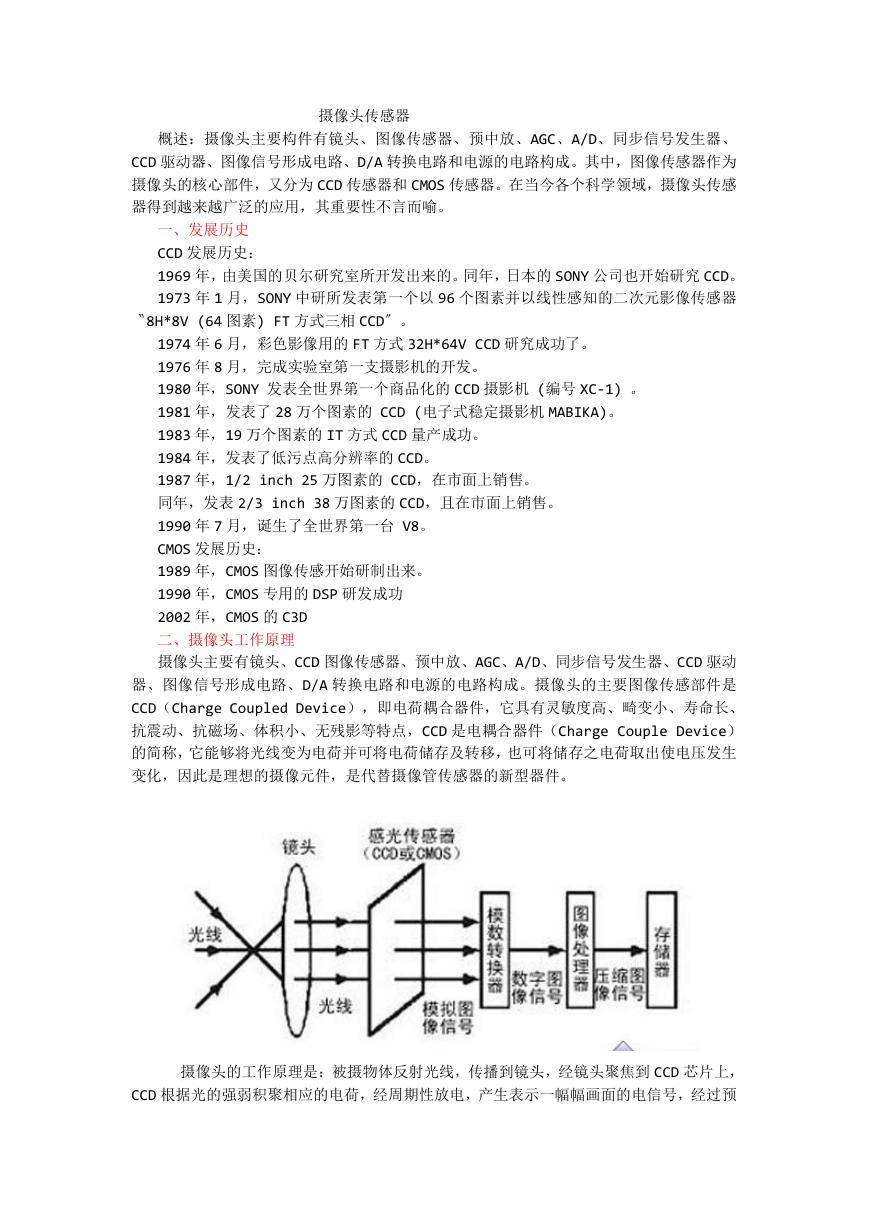 摄像头工作原理.doc
 VL53L0X简要说明(En.FLVL53L00216).pdf
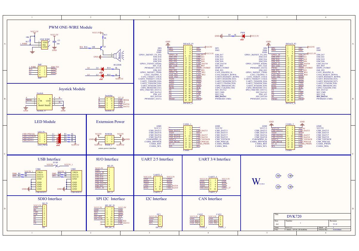 原理图(DVK720-Schematic).pdf
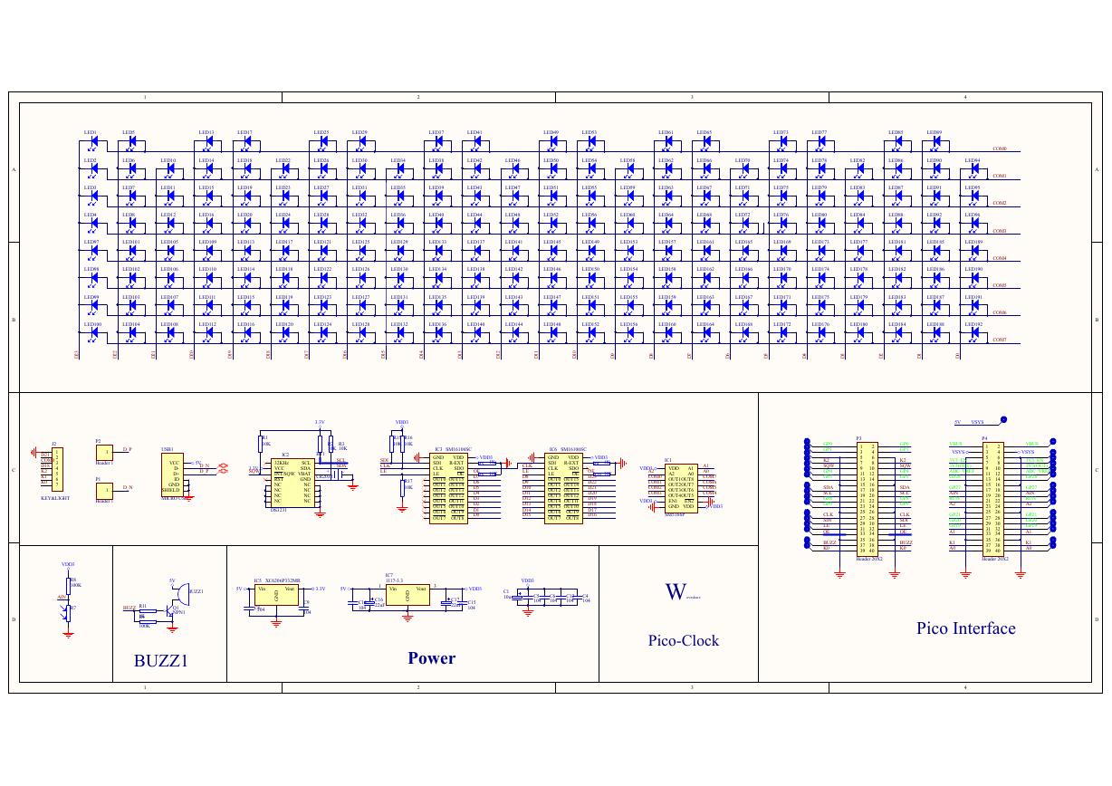 原理图(Pico-Clock-Green-Schdoc).pdf
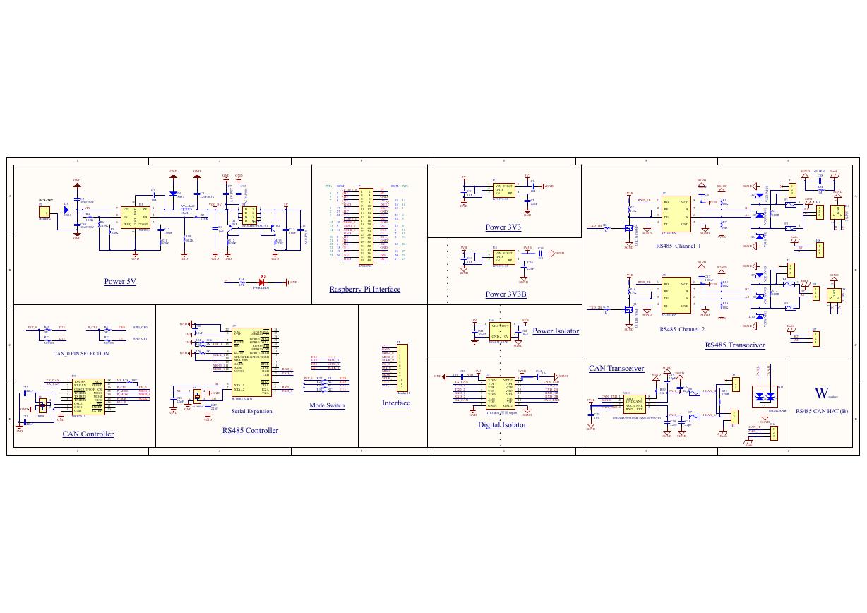 原理图(RS485-CAN-HAT-B-schematic).pdf
 File:SIM7500_SIM7600_SIM7800 Series_SSL_Application Note_V2.00.pdf
 ADS1263(Ads1262).pdf
 原理图(Open429Z-D-Schematic).pdf
 用户手册(Capacitive_Fingerprint_Reader_User_Manual_CN).pdf
 CY7C68013A(英文版)(CY7C68013A).pdf
 TechnicalReference_Dem.pdf
 23-S4P+与IRC5P的差别-ABB喷涂机器人培训.pdf