CEC 2015 优化问题的测试函数.pdf-资料库

Problem Definitions and Evaluation Criteria for the CEC 2015 Competition on Learning-based Real-Parameter Single Objective Optimization J. J. Liang1, B. Y. Qu2, P. N. Suganthan3, Q. Chen4 1School of Electrical Engineering, Zhengzhou University, Zhengzhou, China 2School of Electric and Information Engineering, Zhongyuan University of Technology, Zhengzhou, China 3 School of Electrical and Electronic Engineering, Nanyang Technological University, Singapore 4Facility Design and Instrument Institute, China Aerodynamic Research and Development Center, China liangjing@zzu.edu.cn, qby1984@hotmail.com, epnsugan@ntu.edu.sg, chenqin1980@gmail.com Technical Report 201411A, Computational Intelligence Laboratory, Zhengzhou University, Zhengzhou China Technical Report, Nanyang Technological University, Singapore And November 2014

CEC 2015 Competition on Learning-based Real-Parameter Single Objective Optimization 1. Introduction Single objective optimization algorithms are the basis of the more complex optimization algorithms such as multi-objective, niching, dynamic, constrained optimization algorithms and so on. Research on single objective optimization algorithms influence the development of the optimization branches mentioned above. In the recent years, various kinds of novel optimization algorithms have been proposed to solve real-parameter optimization problems. This special session is devoted to the approaches, algorithms and techniques for solving real parameter single objective optimization without knowing the exact equations of the test functions (i.e. blackbox optimization). We encourage all researchers to test their algorithms on the CEC’15 test suites. The participants are required to send the final results(after submitting their final paper version in March 2015)in the format specified in this technical report to the organizers. The organizers will present an overall analysis and comparison based on these results. We will also use statistical tests on convergence performance to compare algorithms that eventually generate similar final solutions. Papers on novel concepts that help us in understanding problem characteristics are also welcome. Results of 10D and 30D problems are acceptable for the first review submission. However, other dimensional results as specified in the technical report should also be included in the final version, if space permits. Thus, final results for all dimensions in the format introduced in the technical report should be zipped and sent to the organizers after the final version of the paper is submitted. Please note that in this competition error values smaller than 10-8 will be taken as zero. You can download the C, JAVA and Matlab codes for CEC’15 test suite from the website given below: http://www.ntu.edu.sg/home/EPNSugan/index_files/CEC2015/CEC2015.htm This technical report presents the details of benchmark suite used for CEC’15 competition on learning based single objective global optimization. 1

CEC 2015 Competition on Learning-based Real-Parameter Single Objective Optimization 1.1 Introduction to Learning-Based Problems As a relatively new solver for the optimization problems, evolutionary algorithm has attracted the attention of researchers in various fields. When testing the performance of a novel evolutionary algorithm, we always choose a group of benchmark functions and compare the proposed new algorithm with other existing algorithms on these benchmark functions. To obtain fair comparison results and to simplify the experiments, we always set the parameters of the algorithms to be the same for all test functions. In general, specifying different sets of parameters for different test functions is not allowed. Due to this approach, we lose the opportunity to analyze how to adjust the algorithm to solve a specified problem in the most effective manner. As we all know that there is no free lunch and for solving a particular real-world problem, we only need one most effective algorithm. In practice, it is hard to imagine a scenario whereby a researcher or engineer has to solve highly diverse problems at the same time. In other words, a practicing engineer is more likely to solve numerous instances of a particular problem. Under this consideration and by the fact that by shifting the position of the optimum and mildly changing the rotation matrix will not change the properties of the benchmark functions significantly, we propose a set of learning-based benchmark problems. In this competition, the participants are allowed to optimize the parameters of their proposed (hybrid) optimization algorithm for each problem. Although a completely different optimization algorithm might be used for solving each of the 15 problems, this approach is strongly discouraged, as our objective is to develop a highly tunable algorithm to solve diverse instances of real-world problems. In other words, our objective is not to identify the best algorithms for solving each of the 15 synthetic benchmark problems. To test the generalization performance of the algorithm and associated parameters, the competition has two stages: Stage 1: Infinite instances of shifted optima and rotation matrixes can be generated. The participants can optimize the parameters of their proposed algorithms for each problem with these data and write the paper. Adaptive learning methods are also allowed. 2

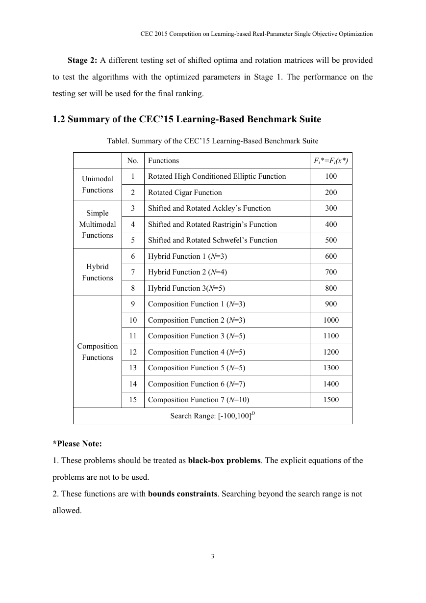
CEC 2015 Competition on Learning-based Real-Parameter Single Objective Optimization Stage 2: A different testing set of shifted optima and rotation matrices will be provided to test the algorithms with the optimized parameters in Stage 1. The performance on the testing set will be used for the final ranking. 1.2 Summary of the CEC’15 Learning-Based Benchmark Suite TableI. Summary of the CEC’15 Learning-Based Benchmark Suite No. Functions Fi*=Fi(x*) Unimodal Functions Simple Multimodal Functions Hybrid Functions Composition Functions 1 2 3 4 5 Rotated High Conditioned Elliptic Function Rotated Cigar Function Shifted and Rotated Ackley’s Function Shifted and Rotated Rastrigin’s Function Shifted and Rotated Schwefel’s Function 6 Hybrid Function 1 (N=3) 7 Hybrid Function 2 (N=4) 8 Hybrid Function 3(N=5) 9 Composition Function 1 (N=3) 10 Composition Function 2 (N=3) 11 Composition Function 3 (N=5) 12 Composition Function 4 (N=5) 13 Composition Function 5 (N=5) 14 Composition Function 6 (N=7) 15 Composition Function 7 (N=10) Search Range: [-100,100]D 100 200 300 400 500 600 700 800 900 1000 1100 1200 1300 1400 1500 *Please Note: 1. These problems should be treated as black-box problems. The explicit equations of the problems are not to be used. 2. These functions are with bounds constraints. Searching beyond the search range is not allowed. 3

CEC 2015 Competition on Learning-based Real-Parameter Single Objective Optimization 1.3 Some Definitions: All test functions are minimization problems defined as following: Min f(x), x  [ x x , 1 2 ,..., x D ] T D: dimensions. o o i iD 1 o o , i i 1 ,..., [ 2 ] T : the shifted global optimum (defined in “shift_data_x.txt”), which is randomly distributed in [-80,80]D. Each function has a shift data for CEC’14. All test functions are shifted to o and scalable. For convenience, the same search ranges are defined for all test functions. Search range: [-100,100]D. Mi: rotation matrix. Different rotation matrices are assigned to each function and each basic function. The variables are divided into subcomponents randomly. The rotation matrix for each subcomponents are generated from standard normally distributed entries by Gram-Schmidt ortho-normalization with condition number c that is equal to 1 or 2. 1.4 Definitions of the Basic Functions 1) High Conditioned Elliptic Function f x ( ) 1 D   i 1  2) Cigar Function 3) Discus Function f 2 x ( )  x 2 1 (10 ) 6 i 1  D 1  x 2 i  D 10 6 i  2 x 2 i (1) (2) f 3 x ( ) 10  6 x 2 1 D i  2 x 2 i (3) 4

CEC 2015 Competition on Learning-based Real-Parameter Single Objective Optimization 4) Rosenbrock’s Function f 4 x ( )  5) Ackley’s Function 1  D i 1  (100( x 2 i  x i 1  2 )  ( x i  1) ) 2 (4) f 5 x ( )   20exp( 0.2  1 D 6) Weierstrass Function D  i 1  x 2 i ) exp(  1 D D  i 1  cos(2 x  i )) 20   e (5) f 6 x ( )  max D k (   i 1  k  0 k [ a cos(2  b x ( k i  0.5))])  D k max  k  0 k [ a cos(2 b  k  0.5)] (6) a=0.5, b=3, kmax=20 7) Griewank’s Function f 7 x ( )  D  i 1  x 2 i 4000  D  i 1  cos( x i i ) 1  (7) 8) Rastrigin’s Function f 8 x ( )  D i 1  2 ( x i  10cos(2 x  i ) 10)  (8) 9) Modified Schwefel’s Function D 418.9829   x ( ) D  f 9 i 1  g z ( i ), z  x i i +4.209687462275036e+002 g z ( i )          z i sin( z i 1/2 ) (500 mod(  z i ,500))sin( 500 mod(  z i ,500) )  ( (mod( z i ,500) 500)sin( mod(  z i ,5 00) 500 )   2  z i 10000 z ( i 10000 500) D 500) D  if z i  500 z if i  500 2 z if i   500 (9) 10) Katsuura Function f 10 x ( )  10 D 2  (1  i 32 j 1  D i 1  j 2 x i  round (2 j x i ) j 2 10 1.2 D )  10 D 2 (10) 5

CEC 2015 Competition on Learning-based Real-Parameter Single Objective Optimization 11) HappyCat Function f 11 x ( )  12) HGBatFunction 1/4 x D 2 i   D  i 1  (0.5   x 2 i  D i 1  D i 1  x i ) / D  0.5 (11) f 12 x ( )  ( D  i 1  x ) 2 2 i  ( 1/2 x i 2 )  D  i 1  (0.5   x 2 i  D i 1  D i 1  x i ) / D  0.5 (12) 13) Expanded Griewank’s plus Rosenbrock’s Function f 13 ( x )  f 7 ( f x x , 4 ( 1 ))  2 f 7 ( f x x , 4 3 ( 2 ))   ... f 7 ( f x ( 4 D 1  , x D ))  f 7 ( f x ( 4 D , x 1 )) (13) 14) Expanded Scaffer’s F6 Function Scaffer’s F6 Function: g x y ( , )  0.5  2 x (sin ( 2  x (1 0.001(  y 2 2 ) 0.5)  y 2 2  )) f 14 ( x )  g x x , ( 1 2 )  g x x , ( 3 2 )   ... g x ( , x D )  g x ( , x 1 ) D D 1  (14) 1.5 Definitions of the CEC’15Learning-Based Benchmark Suite A. 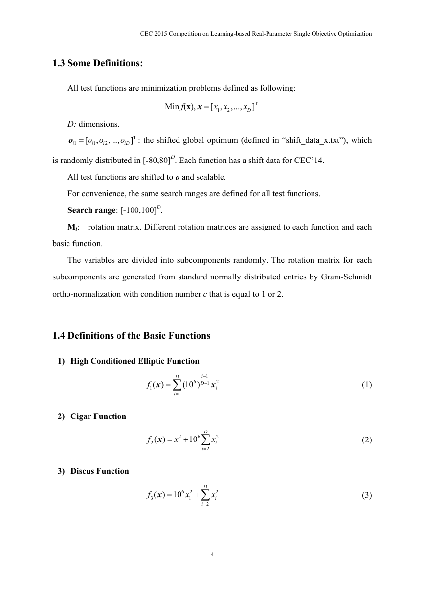Unimodal Functions: 1) Rotated High Conditioned Elliptic Function F 1 ( x )  f 1 ( M 1 ( x o 1  ))  F 1 * (15) Figure 1.3-D map for 2-D function 6

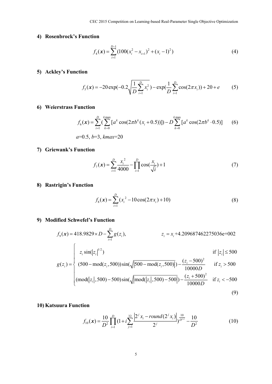
CEC 2015 Competition on Learning-based Real-Parameter Single Objective Optimization Properties:  Unimodal  Non-separable  Quadratic ill-conditioned 2) Rotated Cigar Function F 2 ( x )  f 2 ( M 2 ( x o 2  ))  F 2 * (16) Figure 2. 3-D map for 2-D function Properties:  Unimodal  Non-separable  Smooth but narrow ridge B. Multimodal Functions 3) Shifted and Rotated Ackley’s Function F 3 ( x )  f 5 ( M ( x o 3  )) 3  F 3 * (17) 7

资料库

CEC 2015 优化问题的测试函数.pdf

相关推荐

人工智能

热门标签

最新资料