IEEE CVPR ����
Real-Time Tracking of Non-Rigid Objects using Mean Shift
Dorin Comaniciu Visvanathan Ramesh
Peter Meer
Imaging & Visualization Department
Electrical & Computer Engineering Department
Siemens Corporate Research
Rutgers University
��� College Road East, Princeton, NJ �����
� Brett Road, Piscataway, NJ �����
Abstract
� Mean Shift Analysis
A new method for real-time tracking of non-rigid ob-
jects seen from a moving camera is proposed. The cen-
tral computational module is based on the mean shift
iterations and nds the most probable target position in
the current frame. The dissimilarity between the target
model (its color distribution) and the target candidates
is expressed by a metric derived from the Bhattacharyya
coecient. The theoretical analysis of the approach
shows that it relates to the Bayesian framework while
providing a practical, fast and ecient solution. The
capability of the tracker to handle in real-time partial
occlusions, signicant clutter, and target scale varia-
tions, is demonstrated for several image sequences.
�
Introduction
The ecient tracking of visual features in complex
environments is a challenging task for the vision com-
munity. Real-time applications such as surveillance and
monitoring [��], perceptual user interfaces [�], smart
rooms [��, ��], and video compression [��] all require
the ability to track moving objects. The computational
complexity of the tracker is critical for most applica-
tions, only a small percentage of a system resources be-
ing allocated for tracking, while the rest is assigned to
preprocessing stages or to high-level tasks such as recog-
nition, trajectory interpretation, and reasoning [��].
This paper presents a new approach to the real-time
tracking of non-rigid objects based on visual features
such as color and/or texture, whose statistical distribu-
tions characterize the object of interest. The proposed
tracking is appropriate for a large variety of objects with
dierent color/texture patterns, being robust to partial
occlusions, clutter, rotation in depth, and changes in
camera position. It is a natural application to motion
analysis of the mean shift procedure introduced earlier
[�, �]. The mean shift iterations are employed to nd
the target candidate that is the most similar to a given
target model, with the similarity being expressed by a
metric based on the Bhattacharyya coecient. Vari-
ous test sequences showed the superior tracking perfor-
mance, obtained with low computational complexity.
The paper is organized as follows. Section � presents
and extends the mean shift property. Section � intro-
duces the metric derived from the Bhattacharyya coef-
cient. The tracking algorithm is developed and ana-
lyzed in Section �. Experiments and comparisons are
given in Section �, and the discussions are in Section �.
We dene next the sample mean shift, introduce the
iterative mean shift procedure, and present a new the-
orem showing the convergence for kernels with convex
and monotonic proles. For applications of the mean
shift property in low level vision (ltering, segmenta-
tion) see [�].
�.� Sample Mean Shift
Given a set fxigi=�:::n of n points in the d-
d, the multivariate kernel density
dimensional space R
estimate with kernel K(x) and window radius (band-
width) h, computed in the point x is given by
^f (x) =
�
nhd
n
Xi=�
K x xi
h :
(�)
The minimization of the average global error between
the estimate and the true density yields the multivariate
Epanechnikov kernel [��, p.�� ]
KE(x) = �
� c
�
�
d (d + �)(� kxk�)
if kxk < �
otherwise
(�)
where cd is the volume of the unit d-dimensional sphere.
Another commonly used kernel is the multivariate nor-
mal
KN (x) = (�)d=�exp
�
�kxk� :
(�)
Let us introduce the prole of a kernel K as a func-
tion k : [�;�) ! R such that K(x) = k(kxk�). For
example, according to (�) the Epanechnikov prole is
kE (x) = �
d (d + �)(� x)
if x < �
otherwise
� c
�
(�)
�
and from (�) the normal prole is given by
Employing the prole notation we can write the density
estimate (�) as
kN (x) = (�)d=�exp
k
Xi=�
g(x) = k
�(x) ;
nhd
�
h
n
^fK (x) =
x xi
�
�
x :
�! :
(�)
(�)
We denote
(�)
assuming that the derivative of k exists for all x �
[�;�), except for a nite set of points. A kernel G
can be dened as
G(x) = C g(kxk�);
(�)
�
�
where C is a normalization constant. Then, by taking
the estimate of the density gradient as the gradient of
the density estimate we have
n
�
^rfK (x)r ^fK (x) =
n
h
h
�
�
nhd+�
�!
x xi
�
Xi=�
(x xi) k
�! =
(xi x) g
x xi
nhd+�
i=� xig
�
Pn
�!#�
� x�
h
� ; ( )
�
i=� g
Pn
h
� can be assumed to be
h
xxi
xxi
xxi
=
nhd+�
Xi=�
" n
g
x xi
Xi=�
i=� g
where Pn
h
nonzero. Note that the derivative of the Epanechnikov
prole is the uniform prole, while the derivative of the
normal prole remains a normal.
estimates computed with kernel K in the points (��)
are
:
(��)
^fK =n ^fK(j)oj=�;�::: n ^fK (yj )oj=�;�:::
These densities are only implicitly dened to obtain
^rfK . However we need them to prove the convergence
of the sequences (��) and (��).
Theorem � If the kernel K has a convex and mono-
tonic decreasing prole and the kernel G is dened ac-
cording to (�) and (�), the sequences (��) and (��) are
convergent.
The Theorem � generalizes the convergence shown
in [�], where K was the Epanechnikov kernel, and G
the uniform kernel. Its proof is given in the Appendix.
Note that Theorem � is also valid when we associate to
each data point xi a positive weight wi.
The last bracket in ( ) contains the sample mean
� Bhattacharyya Coecient Based
shift vector
(��)
(��)
and the density estimate at x
xxi
i=� xig
Mh;G(x) Pn
i=� g
Pn
g
Xi=�
^fG(x)
C
nhd
n
xxi
�
h
� x
h
�!
x xi
h
computed with kernel G. Using now (��) and (��), ( )
becomes
^rfK (x) = ^fG(x)
from where it follows that
�=C
h
� Mh;G(x)
Mh;G(x) =
�
h
�=C
^rfK (x)
^fG(x)
:
(��)
(��)
Expression (��) shows that the sample mean shift vec-
tor obtained with kernel G is an estimate of the normal-
ized density gradient obtained with kernel K. This is a
more general formulation of the property rst remarked
by Fukunaga [��, p. ���].
�.� A Sucient Convergence Condition
The mean shift procedure is dened recursively by
computing the mean shift vector Mh;G(x) and trans-
lating the center of kernel G by Mh;G(x).
the sequence of succes-
sive locations of the kernel G, where
Let us denote byyjj=�;�:::
i=� xig
�
yj+� = Pn
�
i=� g
Pn
yj xi
xi
yj
h
h
is the weighted mean at yj computed with kernel G
and y� is the center of the initial kernel. The density
;
j = �; �; : : :
(��)
Metric for Target Localization
The task of nding the target location in the current
frame is formulated as follows. The feature z repre-
senting the color and/or texture of the target model is
assumed to have a density function qz, while the target
candidate centered at location y has the feature dis-
tributed according to pz(y). The problem is then to
nd the discrete location y whose associated density
pz(y) is the most similar to the target density qz.
To dene the similarity measure we take into account
that the probability of classication error in statistical
hypothesis testing is directly related to the similarity
of the two distributions. The larger the probability of
error, the more similar the distributions. Therefore,
(contrary to the hypothesis testing), we formulate the
target location estimation problem as the derivation of
the estimate that maximizes the Bayes error associated
with the model and candidate distributions. For the
moment, we assume that the target has equal prior
probability to be present at any location y in the neigh-
borhood of the previously estimated location.
An entity closely related to the Bayes error is the
Bhattacharyya coecient, whose general form is de-
ned by [� ]
(y) [p(y); q] =Z ppz(y)qz dz :
Properties of the Bhattacharyya coecient such as its
relation to the Fisher measure of information, quality
of the sample estimate, and explicit forms for various
distributions are given in [��, � ].
(��)
Our interest in expression (��) is, however, moti-
vated by its near optimality given by the relationship
to the Bayes error. Indeed, let us denote by and
two sets of parameters for the distributions p and q and
by = (p; q) a set of prior probabilities. If the value
of (��) is smaller for the set than for the set , it
�
�
can be proved [� ] that, there exists a set of priors
for which the error probability for the set is less than
the error probability for the set . In addition, starting
from (��) upper and lower error bounds can be derived
for the probability of error.
The derivation of the Bhattacharyya coecient from
sample data involves the estimation of the densities p
and q, for which we employ the histogram formulation.
Although not the best nonparametric density estimate
[��], the histogram satises the low computational cost
imposed by real-time processing. We estimate the dis-
u=� ^qu = �)
from the m-bin histogram of the target model, while
u=� ^pu = �) is estimated
at a given location y from the m-bin histogram of the
target candidate. Hence, the sample estimate of the
Bhattacharyya coecient is given by
crete density ^q = f^qugu=�:::m (with Pm
^p(y) = f^pu(y)gu=�:::m (withPm
m
^(y) [^p(y); ^q] =
Xu=�p^pu(y)^qu:
(��)
The geometric interpretation of (��) is the cosine of
the angle between the m-dimensional, unit vectors
(��)
Using now (��) the distance between two distribu-
p^p�; : : : ;p ^pm>
tions can be dened as
.
and p^q�; : : : ;p^qm>
d(y) =p� [^p(y); ^q] :
The statistical measure (��) is well suited for the
task of target localization since:
�. It is nearly optimal, due to its link to the Bayes
error. Note that the widely used histogram inter-
section technique [��] has no such theoretical foun-
dation.
�. It imposes a metric structure (see Appendix). The
Bhattacharyya distance [��, p. ] or Kullback di-
vergence [�, p.��] are not metrics since they violate
at least one of the distance axioms.
�. Using discrete densities, (��) is invariant to the
scale of the target (up to quantization eects). His-
togram intersection is scale variant [��].
�. Being valid for arbitrary distributions, the dis-
tance (��) is superior to the Fisher linear discrim-
inant, which yields useful results only for distri-
butions that are separated by the mean-dierence
[��, p.���].
Similar measures were already used in computer vi-
sion. The Cherno and Bhattacharyya bounds have
been employed in [��] to determine the eectiveness of
edge detectors. The Kullback divergence has been used
in [��] for nding the pose of an object in an image.
The next section shows how to minimize (��) as a
function of y in the neighborhood of a given location,
by exploiting the mean shift iterations. Only the distri-
bution of the object colors will be considered, although
the texture distribution can be integrated into the same
framework.
�
� Tracking Algorithm
We assume in the sequel the support of two modules
which should provide (a) detection and localization in
the initial frame of the objects to track (targets) [��, ��],
and (b) periodic analysis of each object to account for
possible updates of the target models due to signicant
changes in color [��].
�.� Color Representation
?
?
i the index b(x
Target Model Let fx
i gi=�:::n be the pixel loca-
tions of the target model, centered at �. We dene a
� ! f� : : : mg which associates to the
function b : R
?
pixel at location x
i ) of the histogram
bin corresponding to the color of that pixel. The prob-
ability of the color u in the target model is derived by
employing a convex and monotonic decreasing kernel
prole k which assigns a smaller weight to the locations
that are farther from the center of the target. The
weighting increases the robustness of the estimation,
since the peripheral pixels are the least reliable, be-
ing often aected by occlusions (clutter) or background.
The radius of the kernel prole is taken equal to one,
by assuming that the generic coordinates x and y are
normalized with hx and hy, respectively. Hence, we can
write
^qu = C
k(kx
?
i k�) [b(x
?
i ) u] ;
(� )
where is the Kronecker delta function. The normal-
ization constant C is derived by imposing the condition
n
Xi=�
u=� ^qu = �, from where
Pm
C =
�
Pn
i=� k(kx
;
?
i k�)
(��)
since the summation of delta functions for u = � : : : m
is equal to one.
Target Candidates Let fxigi=�:::nh
be the pixel
locations of the target candidate, centered at y in the
current frame. Using the same kernel prole k, but with
radius h, the probability of the color u in the target
candidate is given by
y xi
h
�! [b(xi) u] ;
(��)
where Ch is the normalization constant. The radius of
the kernel prole determines the number of pixels (i.e.,
the scale) of the target candidate. By imposing the
nh
Xi=�
^pu(y) = Ch
k
condition that Pm
Ch =
�
u=� ^pu = � we obtain
Pnh
i=� k(k yxi
h k�)
:
(��)
Note that Ch does not depend on y, since the pixel lo-
cations xi are organized in a regular lattice, y being one
of the lattice nodes. Therefore, Ch can be precalculated
for a given kernel and dierent values of h.
�
�.� Distance Minimization
According to Section �, the most probable location
y of the target in the current frame is obtained by min-
imizing the distance (��), which is equivalent to maxi-
mizing the Bhattacharyya coecient ^(y). The search
for the new target location in the current frame starts at
the estimated location ^y� of the target in the previous
frame. Thus, the color probabilities f^pu(^y�)gu=�:::m
of the target candidate at location ^y� in the current
frame have to be computed rst. Using Taylor expan-
sion around the values ^pu(^y�), the Bhattacharyya co-
ecient (��) is approximated as (after some manipula-
tions)
[^p(y); ^q]
m
�
�
Xu=�p^pu(^y�)^qu +
�
�
m
Xu=�
^pu(y)s ^qu
it
the
target
is assumed that
^pu(^y�)
(��)
where
candidate
f^pu(y)gu=�:::m does not change drastically from the
initial f^pu(^y�)gu=�:::m, and that ^pu(^y�) > � for all
Introducing now (��) in (��) we obtain
u = � : : : m.
�!
wik
Xi=�
[b(xi) u]s ^qu
Xu=�p^pu(^y�)^qu+
Xu=�
[^p(y); ^q]
y xi
^pu(^y�)
Ch
�
where
wi =
(��)
(��)
m
�
�
nh
m
h
:
Thus, to minimize the distance (��), the second term
in equation (��) has to be maximized, the rst term
being independent of y. The second term represents
the density estimate computed with kernel prole k at
y in the current frame, with the data being weighted by
wi (��). The maximization can be eciently achieved
based on the mean shift iterations, using the following
algorithm.
Bhattacharyya Coecient [^p(y); ^q] Maximization
Given the distribution f^qugu=�:::m of the target model
and the estimated location ^y� of the target in the pre-
vious frame:
�. Initialize the location of the target in the cur-
rent frame with ^y�, compute the distribution
f^pu(^y�)gu=�:::m, and evaluate
[^p(^y�); ^q] =Pm
u=�p^pu(^y�)^qu :
�. Derive the weights fwigi=�:::nh
�. Based on the mean shift vector, derive the new
according to (��).
location of the target (��)
i=� xiwi g
^y� = Pnh
i=� wi g
Pnh
^y�xi
h
^y�xi
h
�
�
:
(��)
�
Update f^pu(^y�)gu=�:::m, and evaluate
u=�p^pu(^y�)^qu :
[^p(^y�); ^q] =Pm
^y� �
�. While [^p(^y�); ^q] < [^p(^y�); ^q]
Do
� (^y� + ^y�).
�. If k^y� ^y�k < Stop.
Otherwise
Set ^y� ^y� and go to Step �.
The proposed optimization employs the mean shift vec-
tor in Step � to increase the value of the approximated
Bhattacharyya coecient expressed by (��). Since this
operation does not necessarily increase the value of
[^p(y); ^q], the test included in Step � is needed to vali-
date the new location of the target. However, practical
experiments (tracking dierent objects, for long peri-
ods of time) showed that the Bhattacharyya coecient
computed at the location dened by equation (��) was
almost always larger than the coecient corresponding
to ^y�. Less than �:�% of the performed maximizations
yielded cases where the Step � iterations were necessary.
The termination threshold used in Step � is derived
by constraining the vectors representing ^y� and ^y� to
be within the same pixel in image coordinates.
The tracking consists in running for each frame the
optimization algorithm described above. Thus, given
the target model, the new location of the target in the
current frame minimizes the distance (��) in the neigh-
borhood of the previous location estimate.
�.� Scale Adaptation
The scale adaptation scheme exploits the property
of the distance (��) to be invariant to changes in the
object scale. We simply modify the radius h of the
kernel prole with a certain fraction (we used ��%),
let the tracking algorithm to converge again, and choose
the radius yielding the largest decrease in the distance
(��). An IIR lter is used to derive the new radius
based on the current measurements and old radius.
� Experiments
The proposed method has been applied to the task
of tracking a football player marked by a hand-drawn
ellipsoidal region (rst image of Figure �). The se-
quence has ��� frames of ��� ��� pixels each and
the initial normalization constants (determined from
the size of the target model) were (hx; hy) = (��; ��).
The Epanechnikov prole (�) has been used for his-
togram computation, therefore, the mean shift itera-
tions were computed with the uniform prole. The tar-
get histogram has been derived in the RGB space with
�� �� �� bins. The algorithm runs comfortably at
�� fps on a ��� MHz PC, Java implementation.
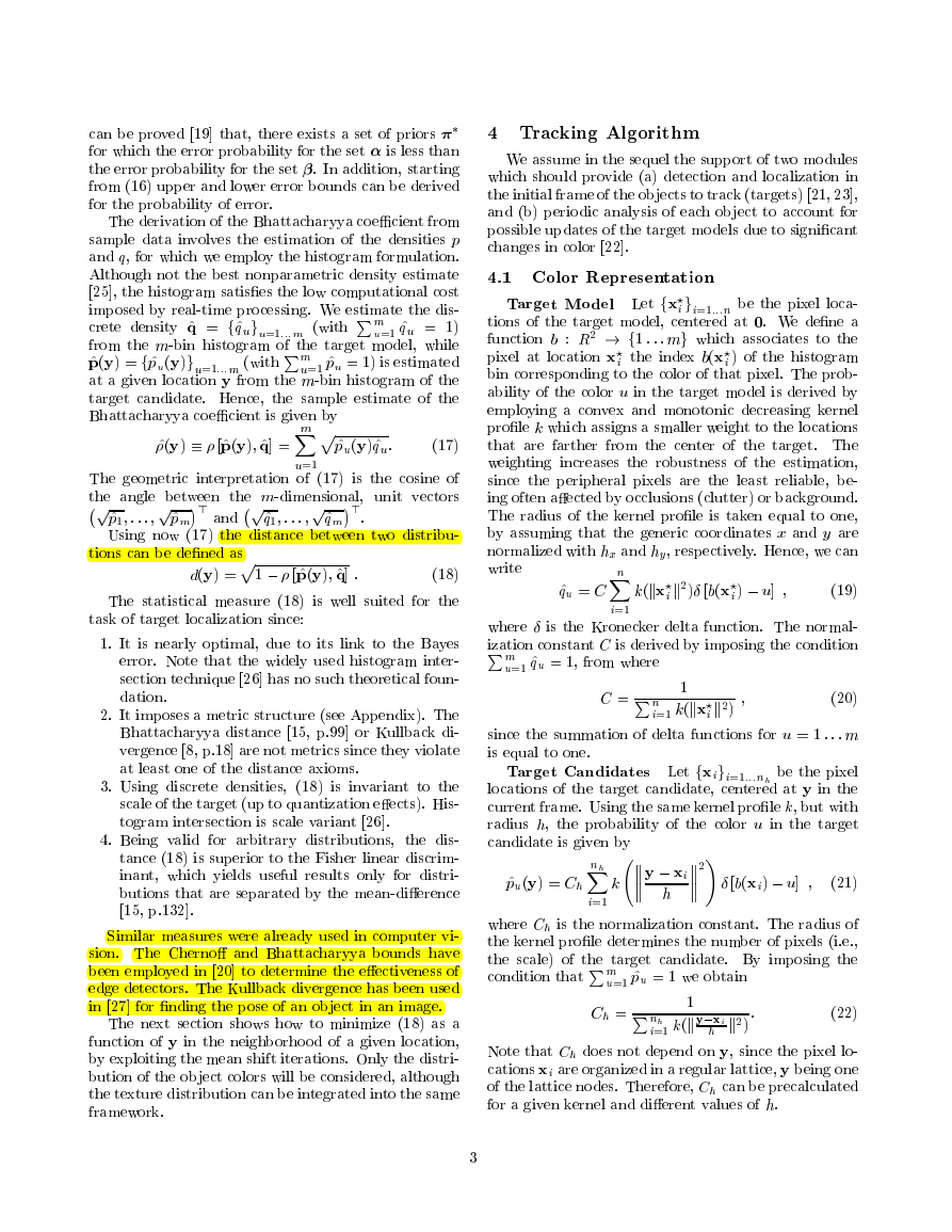
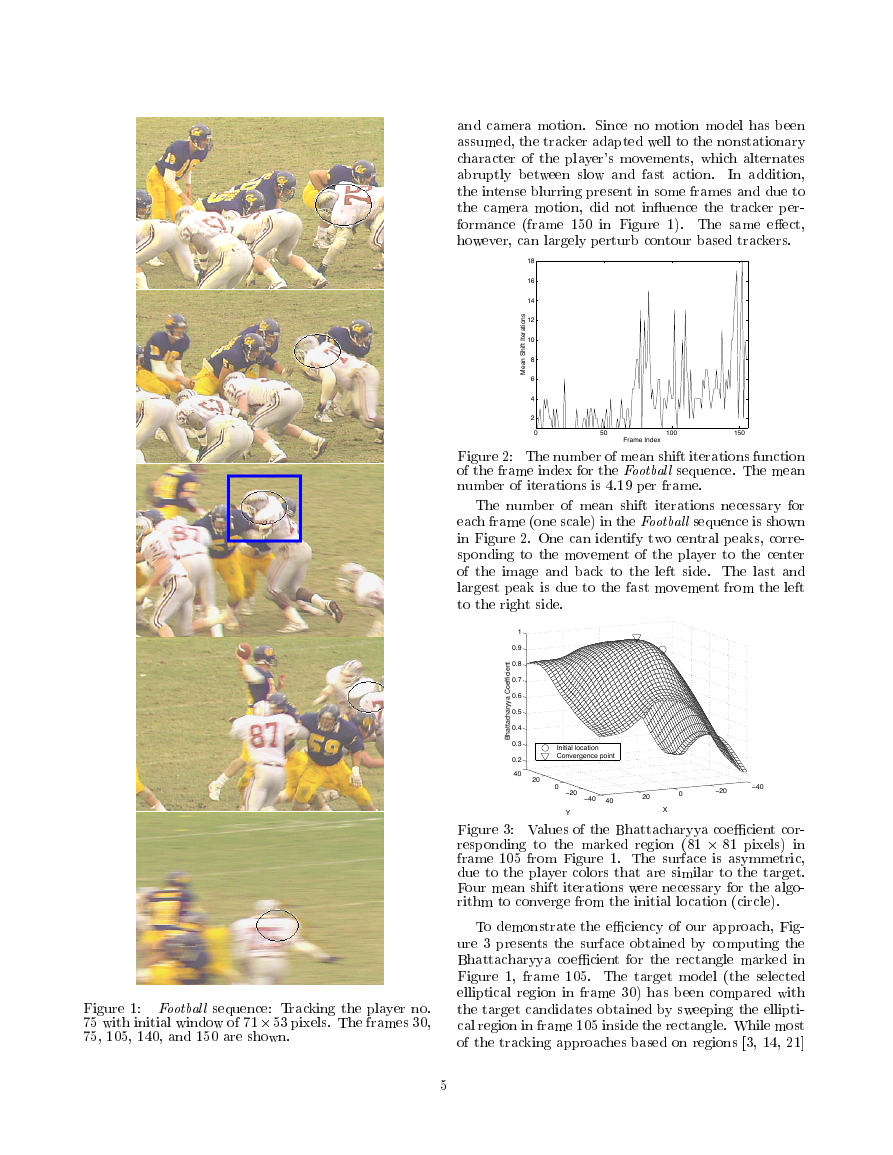
The tracking results are presented in Figure �. The
mean shift based tracker proved to be robust to partial
occlusion, clutter, distractors (frame ��� in Figure �),
�
and camera motion. Since no motion model has been
assumed, the tracker adapted well to the nonstationary
character of the player’s movements, which alternates
abruptly between slow and fast action.
In addition,
the intense blurring present in some frames and due to
the camera motion, did not inuence the tracker per-
formance (frame ��� in Figure �). The same eect,
however, can largely perturb contour based trackers.
s
n
o
i
t
a
r
e
t
I
t
f
i
h
S
n
a
e
M
18
16
14
12
10
8
6
4
2
0
50
Frame Index
100
150
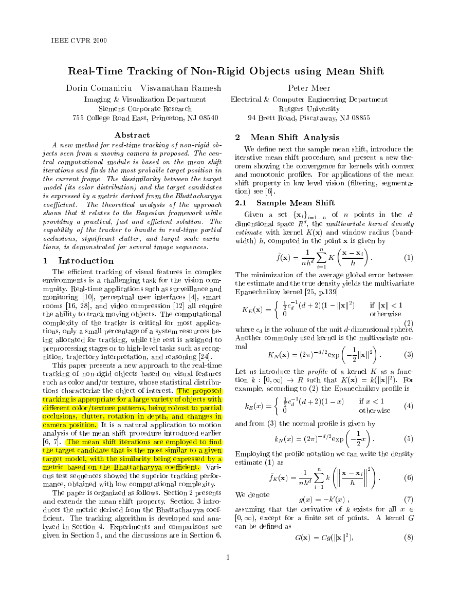
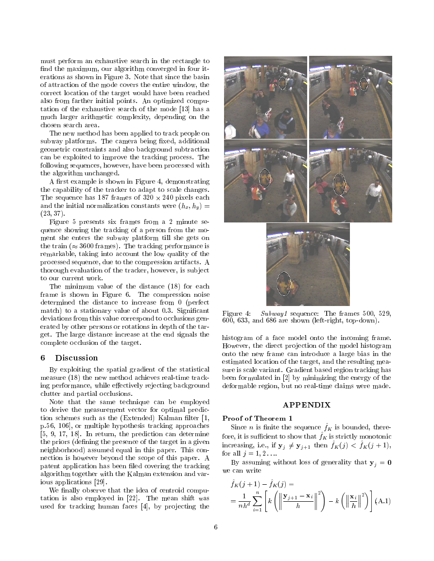
Figure �: The number of mean shift iterations function
of the frame index for the Football sequence. The mean
number of iterations is �:� per frame.
The number of mean shift iterations necessary for
each frame (one scale) in the Football sequence is shown
in Figure �. One can identify two central peaks, corre-
sponding to the movement of the player to the center
of the image and back to the left side. The last and
largest peak is due to the fast movement from the left
to the right side.
t
i
n
e
c
i
f
f
e
o
C
a
y
y
r
a
h
c
a
t
t
a
h
B
1
0.9
0.8
0.7
0.6
0.5
0.4
0.3
0.2
40
Initial location
Convergence point
20
0
−20
Y
−40
40
20
0
X
−20
−40
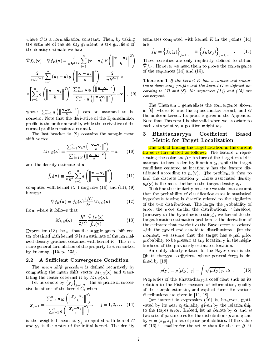
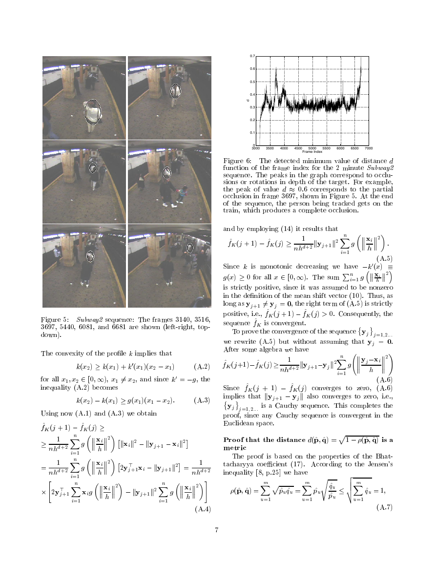
Figure �: Values of the Bhattacharyya coecient cor-
responding to the marked region (�� �� pixels) in
frame ��� from Figure �. The surface is asymmetric,
due to the player colors that are similar to the target.
Four mean shift iterations were necessary for the algo-
rithm to converge from the initial location (circle).
To demonstrate the eciency of our approach, Fig-
ure � presents the surface obtained by computing the
Bhattacharyya coecient for the rectangle marked in
Figure �, frame ���. The target model (the selected
elliptical region in frame ��) has been compared with
the target candidates obtained by sweeping the ellipti-
cal region in frame ��� inside the rectangle. While most
of the tracking approaches based on regions [�, ��, ��]
Figure �: Football sequence: Tracking the player no.
�� with initial window of �� �� pixels. The frames ��,
��, ���, ���, and ��� are shown.
�
�
must perform an exhaustive search in the rectangle to
nd the maximum, our algorithm converged in four it-
erations as shown in Figure �. Note that since the basin
of attraction of the mode covers the entire window, the
correct location of the target would have been reached
also from farther initial points. An optimized compu-
tation of the exhaustive search of the mode [��] has a
much larger arithmetic complexity, depending on the
chosen search area.
The new method has been applied to track people on
subway platforms. The camera being xed, additional
geometric constraints and also background subtraction
can be exploited to improve the tracking process. The
following sequences, however, have been processed with
the algorithm unchanged.
A rst example is shown in Figure �, demonstrating
the capability of the tracker to adapt to scale changes.
The sequence has ��� frames of ��� ��� pixels each
and the initial normalization constants were (hx; hy) =
(��; ��).
Figure � presents six frames from a � minute se-
quence showing the tracking of a person from the mo-
ment she enters the subway platform till she gets on
the train ( ���� frames). The tracking performance is
remarkable, taking into account the low quality of the
processed sequence, due to the compression artifacts. A
thorough evaluation of the tracker, however, is subject
to our current work.
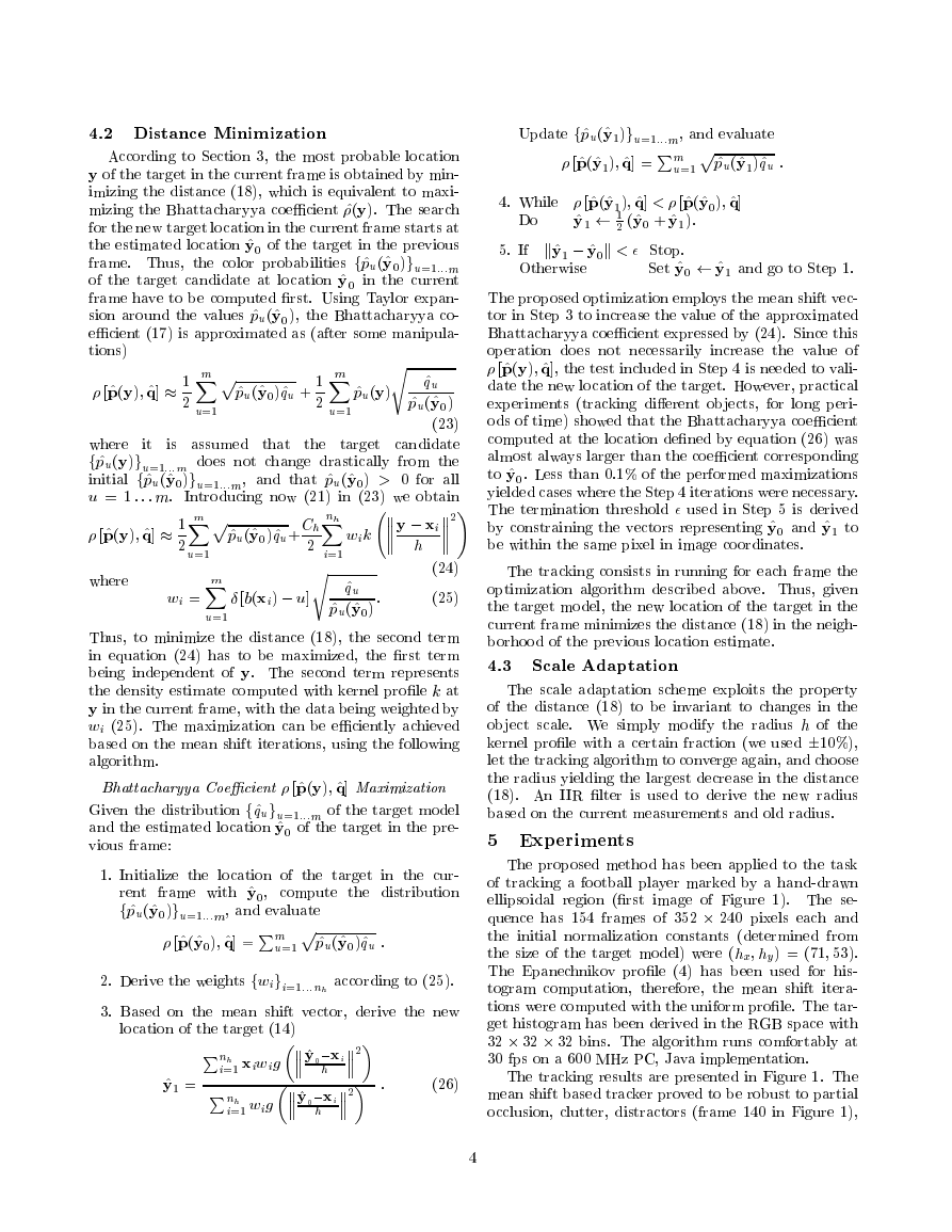
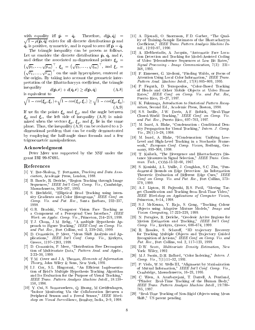
The minimum value of the distance (��) for each
frame is shown in Figure �. The compression noise
determined the distance to increase from � (perfect
match) to a stationary value of about �:�. Signicant
deviations from this value correspond to occlusions gen-
erated by other persons or rotations in depth of the tar-
get. The large distance increase at the end signals the
complete occlusion of the target.
� Discussion
By exploiting the spatial gradient of the statistical
measure (��) the new method achieves real-time track-
ing performance, while eectively rejecting background
clutter and partial occlusions.
Note that the same technique can be employed
to derive the measurement vector for optimal predic-
tion schemes such as the (Extended) Kalman lter [�,
p.��, ���], or multiple hypothesis tracking approaches
[�, , ��, ��]. In return, the prediction can determine
the priors (dening the presence of the target in a given
neighborhood) assumed equal in this paper. This con-
nection is however beyond the scope of this paper. A
patent application has been led covering the tracking
algorithm together with the Kalman extension and var-
ious applications [� ].
We nally observe that the idea of centroid compu-
tation is also employed in [��]. The mean shift was
used for tracking human faces [�], by projecting the
Figure �:
���, ���, and ��� are shown (left-right, top-down).
Subway� sequence: The frames ���, �� ,
histogram of a face model onto the incoming frame.
However, the direct projection of the model histogram
onto the new frame can introduce a large bias in the
estimated location of the target, and the resulting mea-
sure is scale variant. Gradient based region tracking has
been formulated in [�] by minimizing the energy of the
deformable region, but no real-time claims were made.
APPENDIX
Proof of Theorem �
Since n is nite the sequence ^fK is bounded, there-
fore, it is sucient to show that ^fK is strictly monotonic
increasing, i.e., if yj �= yj+� then ^fK (j) < ^fK (j + �),
By assuming without loss of generality that yj = �
for all j = �; � : : :.
we can write
^fK (j + �) ^fK (j) =
=
�
nhd
�
n
Xi=�"k
yj+� xi
h
�! k
xi
h
�# :(A.�)
�
0.7
0.6
0.5
0.4
0.3
0.2
0.1
d
0
3000
3500
4000
4500
5000
Frame Index
5500
6000
6500
7000
Figure �: The detected minimum value of distance d
function of the frame index for the � minute Subway�
sequence. The peaks in the graph correspond to occlu-
sions or rotations in depth of the target. For example,
the peak of value d �:� corresponds to the partial
occlusion in frame �� �, shown in Figure �. At the end
of the sequence, the person being tracked gets on the
train, which produces a complete occlusion.
and by employing (��) it results that
n
�
xi
xi
nhd+�kyj+�k�
^fK (j + �) ^fK(j)
� :
g
h
Xi=�
(A.�)
Since k is monotonic decreasing we have k
�(x)
�
i=� g
g(x) � for all x � [�;�). The sum Pn
h
is strictly positive, since it was assumed to be nonzero
in the denition of the mean shift vector (��). Thus, as
long as yj+� �= yj = �, the right term of (A.�) is strictly
positive, i.e., ^fK (j + �) ^fK (j) > �. Consequently, the
sequence ^fK is convergent.
To prove the convergence of the sequenceyjj=�;�:::
�!
Since ^fK(j + �) ^fK (j) converges to zero, (A.�)
implies that kyj+� yjk also converges to zero, i.e.,
yjj=�;�:::
is a Cauchy sequence. This completes the
proof, since any Cauchy sequence is convergent in the
Euclidean space.
we rewrite (A.�) but without assuming that yj = �.
After some algebra we have
Xi=�
nhd+�kyj+�yjk�
^fK (j+�) ^fK(j)
g
yjxi
(A.�)
�
h
n
metric
Proof that the distance d(^p; ^q) =p� (^p; ^q) is a
The proof is based on the properties of the Bhat-
tacharyya coecient (��). According to the Jensen’s
inequality [�, p.��] we have
(^p; ^q) =
m
Xu=�p^pu ^qu =
m
Xu=�
^pu vuut
^pus ^qu
m
Xu=�
^qu = �;
(A.�)
�
Figure �: Subway� sequence: The frames ����, ����,
�� �, ����, ����, and ���� are shown (left-right, top-
down).
The convexity of the prole k implies that
�(x�)(x� x�)
for all x�; x� � [�;�), x� �= x�, and since k
inequality (A.�) becomes
k(x�) k(x�) + k
(A.�)
� = g, the
k(x�) k(x�) g(x�)(x� x�):
(A.�)
Using now (A.�) and (A.�) we obtain
^fK (j + �) ^fK (j)
nhd+�
�
n
=
�
nhd+�
"�y
>
j+�
n
Xi=�
Xi=�
Xi=�
n
>
xi
xi
�kxik� kyj+� xik�
g
h
g
��y
h
j+�xi kyj+�k� =
� kyj+�k�
g
xig
h
h
Xi=�
xi
xi
n
�#
(A.�)
�
nhd+�
�
with equality i ^p = ^q.
Therefore, d(^p; ^q) =
p� (^p; ^q) exists for all discrete distributions ^p and
^q, is positive, symmetric, and is equal to zero i ^p = ^q.
The triangle inequality can be proven as follows.
Let us consider the discrete distributions ^p, ^q, and ^r,
and dene the associated m-dimensional points p =
, and r =
on the unit hypersphere, centered at
the origin. By taking into account the geometric inter-
pretation of the Bhattacharyya coecient, the triangle
inequality
, q = p^q�; : : : ;p^qm>
p^p�; : : : ;p ^pm>
p^r�; : : : ;p^rm>
is equivalent to
d(^p; ^r) + d(^q; ^r) d(^p; ^q)
(A.�)
q� cos(p; r)+q� cos(q ; r) q� cos(p; q):
(A. )
If we x the points p and q, and the angle between
p and r, the left side of inequality (A. ) is mini-
mized when the vectors p, q, and r lie in the same
plane. Thus, the inequality (A. ) can be reduced to a �-
dimensional problem that can be easily demonstrated
by employing the half-angle sinus formula and a few
trigonometric manipulations.
Acknowledgment
Peter Meer was supported by the NSF under the
grant IRI -��� �.
References
[�] Y. Bar-Shalom, T. Fortmann, Tracking and Data Asso-
ciation, Academic Press, London, � ��.
[�] B. Bascle, R. Deriche, \Region Tracking through Image
Sequences," IEEE Int’l Conf. Comp. Vis., Cambridge,
Massachusetts, ���{���, � �.
[�] S. Bircheld, \Elliptical Head Tracking using inten-
sity Gradients and Color Histograms," IEEE Conf. on
Comp. Vis. and Pat. Rec., Santa Barbara, ���{���,
� �.
[�] G.R. Bradski, \Computer Vision Face Tracking as
a Component of a Perceptual User Interface," IEEE
Work. on Applic. Comp. Vis., Princeton, ���{�� , � �.
[�] T.J. Cham, J.M. Rehg, \A multiple Hypothesis Ap-
proach to Figure Tracking," IEEE Conf. on Comp. Vis.
and Pat. Rec., Fort Collins, vol. �, �� {���, � .
[�] D. Comaniciu, P. Meer, \Mean Shift Analysis and Ap-
plications," IEEE Int’l Conf. Comp. Vis., Kerkyra,
Greece, �� �{����, � .
[�] D. Comaniciu, P. Meer, \Distribution Free Decomposi-
tion of Multivariate Data," Pattern Anal. and Applic.,
�:��{��, � .
[�] T.M. Cover and J.A. Thomas, Elements of Information
Theory, John Wiley & Sons, New York, � �.
[ ] I.J. Cox, S.L. Hingorani, \An Ecient Implementa-
tion of Reid’s Multiple Hypothesis Tracking Algorithm
and Its Evaluation for the Purpose of Visual Tracking,"
IEEE Trans. Pattern Analysis Machine Intell., ��:���{
���, � �.
[��] Y. Cui, S. Samarasekera, Q. Huang, M Greienhagen,
\Indoor Monitoring Via the Collaboration Between a
Peripheral Senson and a Foveal Sensor," IEEE Work-
shop on Visual Surveillance, Bombay, India, �{ , � �.
�
[��] A. Djouadi, O. Snorrason, F.D. Garber, \The Qual-
ity of Training-Sample Estimates of the Bhattacharyya
Coecient," IEEE Trans. Pattern Analysis Machine In-
tell., ��: �{ �, � �.
[��] A. Eleftheriadis, A. Jacquin, \Automatic Face Loca-
tion Detection and Tracking for Model-Assisted Coding
of Video Teleconference Sequences at Low Bit Rates,"
Signal Processing - Image Communication, �(�): ���{
���, � �.
[��] F. Ennesser, G. Medioni, \Finding Waldo, or Focus of
Attention Using Local Color Information," IEEE Trans.
Pattern Anal. Machine Intell., ��(�):���{�� , � �.
[��] P. Fieguth, D. Terzopoulos, \Color-Based Tracking
of Heads and Other Mobile Objects at Video Frame
Rates," IEEE Conf. on Comp. Vis. and Pat. Rec,
Puerto Rico, ��{��, � �.
[��] K. Fukunaga, Introduction to Statistical Pattern Recog-
nition, Second Ed., Academic Press, Boston, � �.
[��] S.S. Intille, J.W. Davis, A.F. Bobick, \Real-Time
Closed-World Tracking," IEEE Conf. on Comp. Vis.
and Pat. Rec., Puerto Rico, � �{���, � �.
[��] M. Isard, A. Blake, \Condensation - Conditional Den-
sity Propagation for Visual Tracking," Intern. J. Comp.
Vis., � (�):�{��, � �.
[��] M. Isard, A. Blake, \ICondensation: Unifying Low-
Level and High-Level Tracking in a Stochastic Frame-
work," European Conf. Comp. Vision, Freiburg, Ger-
many, � �{ ��, � �.
[� ] T. Kailath, \The Divergence and Bhattacharyya Dis-
tance Measures in Signal Selection," IEEE Trans. Com-
mun. Tech., COM-��:��{��, � ��.
[��] S. Konishi, A.L. Yuille, J. Coughlan, S.C. Zhu, \Fun-
damental Bounds on Edge Detection: An Information
Theoretic Evaluation of Dierent Edge Cues," IEEE
Conf. on Comp. Vis. and Pat. Rec., Fort Collins, ���{
�� , � .
[��] A.J. Lipton, H. Fujiyoshi, R.S. Patil, \Moving Tar-
get Classication and Tracking from Real-Time Video,"
IEEE Workshop on Applications of Computer Vision,
Princeton, �{��, � �.
[��] S.J. McKenna, Y. Raja, S. Gong, \Tracking Colour
Objects using Adaptive Mixture Models," Image and
Vision Computing, ��:���{�� , � .
[��] N. Paragios, R. Deriche, \Geodesic Active Regions for
Motion Estimation and Tracking," IEEE Int’l Conf.
Comp. Vis., Kerkyra, Greece, ���{���, � .
[��] R. Rosales, S. Sclaro, \�D trajectory Recovery
for Tracking Multiple Objects and Trajectory Guided
Recognition of Actions," IEEE Conf. on Comp. Vis. and
Pat. Rec., Fort Collins, vol. �, ���{���, � .
[��] D.W. Scott, Multivariate Density Estimation, New
York: Wiley, � �.
[��] M.J. Swain, D.H. Ballard, \Color Indexing," Intern. J.
Comp. Vis., �(�):��{��, � �.
[��] P. Viola, W.M. Wells III, \Alignment by Maximization
of Mutual Information," IEEE Int’l Conf. Comp. Vis.,
Cambridge, Massachusetts, ��{��, � �.
[��] C. Wren, A. Azarbayejani, T. Darrell, A. Pentland,
\Pnder: Real-Time Tracking of the Human Body,"
IEEE Trans. Pattern Analysis Machine Intell., � :���{
���, � �.
[� ] \Real-Time Tracking of Non-Rigid Objects using Mean
Shift," US patent pending.
�


 2023年江西萍乡中考道德与法治真题及答案.doc
 2012年重庆南川中考生物真题及答案.doc
 2013年江西师范大学地理学综合及文艺理论基础考研真题.doc
 2020年四川甘孜小升初语文真题及答案I卷.doc
 2020年注册岩土工程师专业基础考试真题及答案.doc
 2023-2024学年福建省厦门市九年级上学期数学月考试题及答案.doc
 2021-2022学年辽宁省沈阳市大东区九年级上学期语文期末试题及答案.doc
 2022-2023学年北京东城区初三第一学期物理期末试卷及答案.doc
 2018上半年江西教师资格初中地理学科知识与教学能力真题及答案.doc
 2012年河北国家公务员申论考试真题及答案-省级.doc
 2020-2021学年江苏省扬州市江都区邵樊片九年级上学期数学第一次质量检测试题及答案.doc
 2022下半年黑龙江教师资格证中学综合素质真题及答案.doc