Cover
Title
Copyright
Dedication
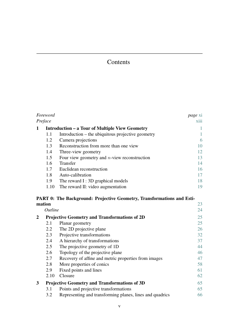
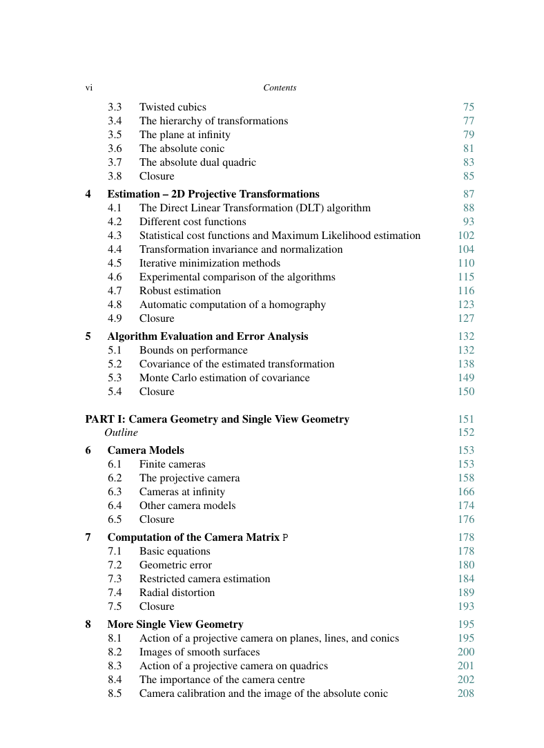
Contents
Foreword
Preface
1 Introduction – a Tour of Multiple View Geometry
1.1 Introduction – the ubiquitous projective geometry
1.1.1 Affine and Euclidean Geometry
1.2 Camera projections
1.3 Reconstruction from more than one view
1.4 Three-view geometry
1.5 Four view geometry and n-view reconstruction
1.6 Transfer
1.7 Euclidean reconstruction
1.8 Auto-calibration
1.9 The reward I : 3D graphical models
1.10 The reward II: video augmentation
Part 0 The Background: Projective Geometry, Transformations and Estimation
Outline
2 Projective Geometry and Transformations of 2D
2.1 Planar geometry
2.2 The 2D projective plane
2.2.1 Points and lines
2.2.2 Ideal points and the line at infinity
2.2.3 Conics and dual conics
2.3 Projective transformations
2.3.1 Transformations of lines and conics
2.4 A hierarchy of transformations
2.4.1 Class I: Isometries
2.4.2 Class II: Similarity transformations
2.4.3 Class III: Affine transformations
2.4.4 Class IV: Projective transformations
2.4.5 Summary and comparison
2.4.6 Decomposition of a projective transformation
2.4.7 The number of invariants
2.5 The projective geometry of 1D
2.6 Topology of the projective plane
2.7 Recovery of affine and metric properties from images
2.7.1 The line at infinity
2.7.2 Recovery of affine properties from images
2.7.3 The circular points and their dual
2.7.4 Angles on the projective plane
2.7.5 Recovery of metric properties from images
2.8 More properties of conics
2.8.1 The pole–polar relationship
2.8.2 Classification of conics
2.9 Fixed points and lines
2.10 Closure
2.10.1 The literature
2.10.2 Notes and exercises
3 Projective Geometry and Transformations of 3D
3.1 Points and projective transformations
3.2 Representing and transforming planes, lines and quadrics
3.2.1 Planes
3.2.2 Lines
3.2.3 Quadrics and dual quadrics
3.2.4 Classification of quadrics
3.3 Twisted cubics
3.4 The hierarchy of transformations
3.4.1 The screw decomposition
3.5 The plane at infinity
3.6 The absolute conic
3.7 The absolute dual quadric
3.8 Closure
3.8.1 The literature
3.8.2 Notes and exercises
4 Estimation – 2D Projective Transformations
4.1 The Direct Linear Transformation (DLT) algorithm
4.1.1 Over-determined solution
4.1.2 Inhomogeneous solution
4.1.3 Degenerate configurations
4.1.4 Solutions from lines and other entities
4.2 Different cost functions
4.2.1 Algebraic distance
4.2.2 Geometric distance
4.2.3 Reprojection error – both images
4.2.4 Comparison of geometric and algebraic distance
4.2.5 Geometric interpretation of reprojection error
4.2.6 Sampson error
Linear cost function
4.2.7 Another geometric interpretation
4.3 Statistical cost functions and Maximum Likelihood estimation
4.4 Transformation invariance and normalization
4.4.1 Invariance to image coordinate transformations
4.4.2 Non-invariance of the DLT algorithm
4.4.3 Invariance of geometric error
4.4.4 Normalizing transformations
4.5 Iterative minimization methods
A word about parametrization
Function specification
Initialization
Iteration methods
4.6 Experimental comparison of the algorithms
4.7 Robust estimation
4.7.1 RANSAC
4.7.2 Robust Maximum Likelihood estimation
4.7.3 Other robust algorithms
4.8 Automatic computation of a homography
4.8.1 Application domain
4.8.2 Implementation and run details
4.9 Closure
4.9.1 The literature
4.9.2 Notes and exercises
5 Algorithm Evaluation and Error Analysis
5.1 Bounds on performance
5.1.1 Error in one image
5.1.2 Error in both images
5.1.3 Optimal estimators (MLE)
5.1.4 Determining the correct convergence of an algorithm
5.2 Covariance of the estimated transformation
5.2.1 Forward propagation of covariance
5.2.2 Backward propagation of covariance
5.2.3 Over-parametrization
5.2.4 Application and examples
5.2.5 Error in both images
5.2.6 Using the covariance matrix in point transfer
5.3 Monte Carlo estimation of covariance
5.4 Closure
5.4.1 The literature
5.4.2 Notes and exercises
Part I Camera Geometry and Single View Geometry
Outline
6 Camera Models
6.1 Finite cameras
6.2 The projective camera
6.2.1 Camera anatomy
6.2.2 Action of a projective camera on points
6.2.3 Depth of points
6.2.4 Decomposition of the camera matrix
6.2.5 Euclidean vs projective spaces
6.3 Cameras at infinity
6.3.1 Affine cameras
6.3.2 Error in employing an affine camera
6.3.3 Decomposition of P…
6.3.4 A hierarchy of affine cameras
6.3.5 More properties of the affine camera
6.3.6 General cameras at infinity
6.4 Other camera models
6.4.1 Pushbroom cameras
6.4.2 Line cameras
6.5 Closure
6.5.1 The literature
6.5.2 Notes and exercises
7 Computation of the Camera Matrix P
7.1 Basic equations
7.2 Geometric error
7.2.1 Geometric interpretation of algebraic error
7.2.2 Estimation of an affine camera
7.3 Restricted camera estimation
Experimental evaluation
7.4 Radial distortion
7.5 Closure
7.5.1 The literature
7.5.2 Notes and exercises
8 More Single View Geometry
8.1 Action of a projective camera on planes, lines, and conics
8.1.1 On planes
8.1.2 On lines
8.1.3 On conics
8.2 Images of smooth surfaces
8.3 Action of a projective camera on quadrics
8.4 The importance of the camera centre
8.4.1 Moving the image plane
8.4.2 Camera rotation
8.4.3 Applications and examples
8.4.4 Projective (reduced) notation
8.4.5 Moving the camera centre
8.5 Camera calibration and the image of the absolute conic
8.5.1 The image of the absolute conic
8.5.2 Orthogonality and Omega
8.6 Vanishing points and vanishing lines
8.6.1 Vanishing points
A note on computing vanishing points
8.6.2 Vanishing lines
Computing vanishing lines
8.6.3 Orthogonality relationships amongst vanishing points and lines
8.7 Affine 3D measurements and reconstruction
8.8 Determining camera calibration K from a single view
8.8.1 The geometry of the constraints
8.9 Single view reconstruction
8.10 The calibrating conic
Orthogonality and the calibrating conic
8.11 Closure
8.11.1 The literature
8.11.2 Notes and exercises
Part II Two-View Geometry
Outline
9 Epipolar Geometry and the Fundamental Matrix
9.1 Epipolar geometry
9.2 The fundamental matrix F
9.2.1 Geometric derivation
9.2.2 Algebraic derivation
9.2.3 Correspondence condition
9.2.4 Properties of the fundamental matrix
9.2.5 The epipolar line homography
9.3 Fundamental matrices arising from special motions
9.3.1 Pure translation
9.3.2 Pure planar motion
9.4 Geometric representation of the fundamental matrix
9.4.1 Pure planar motion
9.5 Retrieving the camera matrices
9.5.1 Projective invariance and canonical cameras
9.5.2 Projective ambiguity of cameras given F
9.5.3 Canonical cameras given F
9.6 The essential matrix
9.6.1 Properties of the essential matrix
9.6.2 Extraction of cameras from the essential matrix
9.6.3 Geometrical interpretation of the four solutions
9.7 Closure
9.7.1 The literature
9.7.2 Notes and exercises
10 3D Reconstruction of Cameras and Structure
10.1 Outline of reconstruction method
10.2 Reconstruction ambiguity
10.3 The projective reconstruction theorem
10.4 Stratified reconstruction
10.4.1 The step to affine reconstruction
Translational motion
Scene constraints
The infinite homography
One of the cameras is affine
10.4.2 The step to metric reconstruction
10.4.3 Direct metric reconstruction using Omega
10.5 Direct reconstruction – using ground truth
10.6 Closure
10.6.1 The literature
10.6.2 Notes and exercises
11 Computation of the Fundamental Matrix F
11.1 Basic equations
11.1.1 The singularity constraint
11.1.2 The minimum case – seven point correspondences
11.2 The normalized 8-point algorithm
11.3 The algebraic minimization algorithm
11.3.1 Iterative estimation
11.4 Geometric distance
11.4.1 The Gold Standard method
11.4.2 Parametrization of rank-2 matrices
11.4.3 First-order geometric error (Sampson distance)
11.5 Experimental evaluation of the algorithms
11.5.1 Recommendations
11.6 Automatic computation of F
11.7 Special cases of F-computation
11.7.1 Pure translational motion
11.7.2 Planar motion
11.7.3 The calibrated case
11.8 Correspondence of other entities
11.9 Degeneracies
11.9.1 Points on a ruled quadric
11.9.2 Points on a plane
11.9.3 No translation
11.10 A geometric interpretation of F-computation
11.11 The envelope of epipolar lines
11.11.1 Verification of epipolar line covariance
11.12 Image rectification
11.12.1 Mapping the epipole to infinity
11.12.2 Matching transformations
11.12.3 Algorithm outline
11.12.4 Affine rectification
11.13 Closure
11.13.1 The literature
11.13.2 Notes and exercises
12 Structure Computation
12.1 Problem statement
12.2 Linear triangulation methods
12.3 Geometric error cost function
12.4 Sampson approximation (first-order geometric correction)
12.5 An optimal solution
12.5.1 Reformulation of the minimization problem
12.5.2 Details of the minimization
12.5.3 Local minima
12.5.4 Evaluation on real images
12.6 Probability distribution of the estimated 3D point
12.7 Line reconstruction
12.8 Closure
12.8.1 The literature
12.8.2 Notes and exercises
13 Scene planes and homographies
13.1 Homographies given the plane and vice versa
13.1.1 Homographies compatible with epipolar geometry
13.2 Plane induced homographies given F and image correspondences
13.2.1 Three points
13.2.2 A point and line
13.3 Computing F given the homography induced by a plane
13.4 The infinite homography H…
13.5 Closure
13.5.1 The literature
13.5.2 Notes and exercises
14 Affine Epipolar Geometry
14.1 Affine epipolar geometry
14.2 The affine fundamental matrix
14.2.1 Derivation
14.2.2 Properties
14.3 Estimating FA from image point correspondences
14.3.1 The linear algorithm
14.3.2 The Gold Standard algorithm
14.3.3 The minimal configuration
14.4 Triangulation
14.5 Affine reconstruction
14.6 Necker reversal and the bas-relief ambiguity
14.7 Computing the motion
14.8 Closure
14.8.1 The literature
14.8.2 Notes and exercises
Part III Three-View Geometry
Outline
16 Computation of the Trifocal Tensor T
15 The Trifocal Tensor
15.1 The geometric basis for the trifocal tensor
15.1.1 Homographies induced by a plane
15.1.2 Point and line incidence relations
15.1.3 Epipolar lines
15.1.4 Extracting the fundamental matrices
15.1.5 Retrieving the camera matrices
15.2 The trifocal tensor and tensor notation
15.2.1 The trilinearities
15.3 Transfer
15.3.1 Point transfer using fundamental matrices
15.3.2 Point transfer using the trifocal tensor
15.3.3 Line transfer using the trifocal tensor
15.4 The fundamental matrices for three views
15.4.1 Uniqueness of camera matrices given three fundamental matrices
15.4.2 Computation of camera matrices from three fundamental matrices
15.4.3 Camera matrices compatible with two fundamental matrices
15.5 Closure
15.5.1 The literature
15.5.2 Notes and exercises
16.1 Basic equations
16.1.1 The internal constraints
16.1.2 The minimum case – 6 point correspondences
16.2 The normalized linear algorithm
How to represent lines
Normalization
16.3 The algebraic minimization algorithm
Retrieving the epipoles
Algebraic minimization
Iterative method
16.4 Geometric distance
16.4.1 The Gold Standard method for the trifocal tensor
16.4.2 Parametrization of the trifocal tensor
16.4.3 First-order geometric error (Sampson distance)
16.5 Experimental evaluation of the algorithms
16.5.1 Results and recommendations
16.6 Automatic computation of T
16.7 Special cases of T -computation
16.7.1 Computing T… from a plane plus parallax
16.7.2 Lines specified by several points
16.8 Closure
16.8.1 The literature
16.8.2 Notes and exercises
Part IV N-View Geometry
Outline
17 N-Linearities and Multiple View Tensors
17.1 Bilinear relations
17.1.1 Epipoles as tensors
17.1.2 Affine specialization
17.2 Trilinear relations
17.2.1 Trifocal point relations
17.2.2 Trifocal line relations
17.2.3 Relations between two views and the trifocal tensor
17.2.4 Affine trifocal tensor
17.3 Quadrilinear relations
17.4 Intersections of four planes
17.5 Counting arguments
17.5.1 Affine cameras
17.5.2 Knowing four coplanar points – plane plus parallax
17.6 Number of independent equations
17.7 Choosing equations
17.8 Closure
17.8.1 The literature
17.8.2 Notes and exercises
18 N-View Computational Methods
18.1 Projective reconstruction – bundle adjustment
18.2 Affine reconstruction – the factorization algorithm
18.2.1 Affine multiple view tensors
18.2.2 Triangulation and reprojection using subspaces
18.2.3 Affine Reconstruction by Alternation
18.3 Non-rigid factorization
18.3.1 Subspaces and tensors
18.3.2 Recovering the camera motion
18.4 Projective factorization
18.4.1 Choosing the depths
18.4.2 What is being minimized?
18.4.3 Normalizing the depths
18.4.4 Normalizing the image coordinates
18.4.5 When is the assumption… = 1 reasonable?
18.5 Projective reconstruction using planes
18.5.1 Direct solution for structure and translation
18.5.2 Direct motion estimation
18.6 Reconstruction from sequences
18.7 Closure
18.7.1 Literature
18.7.2 Notes and exercises
19 Auto-Calibration
19.1 Introduction
19.2 Algebraic framework and problem statement
19.3 Calibration using the absolute dual quadric
19.3.1 Linear solutions for Q… from a set of images
19.3.2 Non-linear solutions for Q…
19.3.3 Iterative methods
19.3.4 A counting argument
19.3.5 Limitations of the absolute quadric approach to calibration
19.4 The Kruppa equations
19.5 A stratified solution
19.5.1 Affine reconstruction – determining Pi…
19.5.2 Affine to metric conversion – determining K given Pi…
19.5.3 The ambiguities in using the infinite homography relation
19.6 Calibration from rotating cameras
19.7 Auto-calibration from planes
19.8 Planar motion
19.9 Single axis rotation – turntable motion
19.10 Auto-calibration of a stereo rig
19.11 Closure
19.11.1 The literature
19.11.2 Notes and exercises
20 Duality
20.1 Carlsson–Weinshall duality
20.1.1 Dual algorithms
20.1.2 Justification of the algorithm
20.2 Reduced reconstruction
20.2.1 The reduced fundamental matrix
20.2.2 Computation of the reduced fundamental matrix
20.2.3 Retrieving reduced camera matrices
20.2.4 Solving for six points in three views
20.2.5 Six points in n views
20.2.6 Seven points in n views
20.2.7 Performance issues
20.3 Closure
20.3.1 The literature
20.3.2 Notes and Exercises
21 Cheirality
21.1 Quasi-affine transformations
21.2 Front and back of a camera
21.3 Three-dimensional point sets
21.4 Obtaining a quasi-affine reconstruction
21.5 Effect of transformations on cheirality
21.6 Orientation
21.7 The cheiral inequalities
Solving the cheiral inequalities
Summary of the algorithm
Bounding the plane at infinity
21.8 Which points are visible in a third view
21.9 Which points are in front of which
21.10 Closure
21.10.1 The literature
22 Degenerate Configurations
22.1 Camera resectioning
22.1.1 Ambiguity in 2D – Chasles’ theorem
22.1.2 Ambiguity for 3D cameras
22.2 Degeneracies in two views
22.2.1 Examples ambiguity
22.3 Carlsson–Weinshall duality
22.3.1 Single view ambiguity
22.3.2 Two-view ambiguity
22.4 Three-view critical configurations
Points in a plane
Points on a twisted cubic
General three-view ambiguity
22.5 Closure
22.5.1 The literature
22.5.2 Notes and exercises
Part V Appendices
Appendix 1 Tensor Notation
A1.1 The tensor…
A1.2 The trifocal tensor
Appendix 2 Gaussian (Normal) and Chi Distributions
A2.1 Gaussian probability distribution
A2.2 Chi distribution
Appendix 3 Parameter Estimation
A3.1 Bias
A3.2 Variance of an estimator
A3.3 The posterior distribution
A3.4 Estimation of corrected measurements
A3.5 Notes and exercises
Appendix 4 Matrix Properties and Decompositions
A4.1 Orthogonal matrices
A4.1.1 Givens rotations and RQ decomposition
A4.1.2 Householder matrices and QR decomposition
A4.2 Symmetric and skew-symmetric matrices
A4.2.1 Positive-definite symmetric matrices
A4.3 Representations of rotation matrices
A4.3.1 Rotations in n-dimensions
A4.3.2 Rotations in 3-dimensions
A4.3.3 Quaternions
A4.4 Singular value decomposition
Appendix 5 Least-squares Minimization
A5.1 Solution of linear equations
A5.2 The pseudo-inverse
A5.2.1 Linear least-squares using normal equations
A5.3 Least-squares solution of homogeneous equations
A5.4 Least-squares solution to constrained systems
A5.4.1 More constrained minimization
A5.4.2 Yet another minimization problem
Appendix 6 Iterative Estimation Methods
A6.1 Newton iteration
A6.2 Levenberg–Marquardt iteration
A6.3 A sparse Levenberg–Marquardt algorithm
A6.3.1 Partitioning the parameters in the LM method
A6.3.2 Covariance
A6.3.3 General sparse LM method
A6.4 Application of sparse LM to 2D homography estimation
A6.4.1 Computation of the covariance
A6.5 Application of sparse LM to fundamental matrix estimation
A6.6 Application of sparse LM to multiple image bundle adjustment
A6.7 Sparse methods for equation solving
A6.7.1 Banded structure in bundle-adjustment
A6.7.2 Solution of symmetric linear equations
A6.7.3 Solution of sparse symmetric linear systems
A6.8 Robust cost functions
A6.8.1 Properties of the different cost functions
A6.8.2 Performance of the different cost functions
A6.9 Parametrization
A6.9.1 Parametrization of 3D rotations
A6.9.2 Parametrization of homogeneous vectors
A6.9.3 Parametrization of the n-sphere
A6.10 Notes and exercises
Appendix 7 Some Special Plane Projective Transformations
A7.1 Conjugate rotations
A7.2 Planar homologies
A7.3 Elations
A7.4 Perspectivities
Bibliography
Index







 2023年江西萍乡中考道德与法治真题及答案.doc
 2012年重庆南川中考生物真题及答案.doc
 2013年江西师范大学地理学综合及文艺理论基础考研真题.doc
 2020年四川甘孜小升初语文真题及答案I卷.doc
 2020年注册岩土工程师专业基础考试真题及答案.doc
 2023-2024学年福建省厦门市九年级上学期数学月考试题及答案.doc
 2021-2022学年辽宁省沈阳市大东区九年级上学期语文期末试题及答案.doc
 2022-2023学年北京东城区初三第一学期物理期末试卷及答案.doc
 2018上半年江西教师资格初中地理学科知识与教学能力真题及答案.doc
 2012年河北国家公务员申论考试真题及答案-省级.doc
 2020-2021学年江苏省扬州市江都区邵樊片九年级上学期数学第一次质量检测试题及答案.doc
 2022下半年黑龙江教师资格证中学综合素质真题及答案.doc