Survival Analysis in R
David Diez
This document is intended to assist an individual who has familiarity with R and who is taking a
survival analysis course. Specifically, this was constructed for a biostatistics course at UCLA. Many
theoretical details have been intentionally omitted for brevity; it is assumed the reader is familiar
with the theory of the topics presented. Likewise, it is assumed the reader has basic understanding
of R including working with data frames, vectors, matrices, plotting, and linear model fitting and
interpretation.
Functions that are introduced will only have the key arguments mentioned and discussed. Most
functions have several other (optional) arguments, however, many of these will not be useful for
an introductory course. The functions, with the exception of those I wrote, have well-written
descriptions that specify each of the potential arguments and their use. The functions I have
written include documentation on the following web site:
Ideally, this survival analysis document would be printed front-to-back and bound like a book. No
topics run over two pages and those that are two pages would then be on opposing pages, making
a topic’s introduction available without the need to flip back and forth between pages (unless the
reader forgets a previous topic, then some flipping may be necessary). A more thorough look at
Cox PH models beyond what is discussed here is available in a guide constructed by John Fox,
which is listed in the References.
Table of Contents
Topic
Packages and data sets
Survival objects
Kaplan-Meier estimate
Confidence bands
Cumulative hazard function
Mean and median estimates
Tests for two or more samples
Cox PH models, contant covariates
Cox PH models, time-dependent covariates
Accelerated failure-time models
References
Page
2
3
4-5
6
7
8
9
10-11
12-13
14-15
16
1
�
R packages :: survival & KMsurv :: The package survival is used in each example
in this document. Every data set used is found in the package KMsurv, which are the data sets
from Klein and Moeschberger’s book. To obtain one or both of these packages (if they were not
previously installed), use
> install.packages(’survival’)
> install.packages(’KMsurv’)
To load the libraries, use
> library(survival)
> library(KMsurv)
To view available data sets, use library(help=KMsurv). To load a data set, use the function
data():
> data(aids)
> aids
infect induct adult
1
1
0.00
0.25
5.00
6.75
7.00
7.25
0.75
0.25
0
0
1
2
...
294
295
The ’...’ denotes output omitted for brevity. Occasionally the ’...’ will itself be omitted. If
the packages survival and KMsurv are both loaded, typing in the sample code in this document’s
examples will allow the reader to reproduce the results. [[ As mentioned, this assumes the libraries
are loaded. Also, any variables already in the workspace with names common with any commands,
variables, or column names in the examples must be removed using rm() to ensure the examples
will run. ]]
To make columns available for use as variables, use attach():
> attach(aids)
> infect
[1] 0.00 0.25 0.75 0.75 0.75 1.00 1.00 1.00 1.00 1.25 1.25 1.25 1.25 1.50
...
[281] 5.25 5.25 5.50 5.50 5.50 5.75 6.00 6.00 6.25 6.25 6.50 6.75 6.75 7.00
[295] 7.25
Detaching the data set when done is a good habit and can prevent errors within R (since two data
sets may have common column names):
> detach(aids)
2
�
Survival object :: Surv(time, time2, event, type) :: Before complex func-
tions may be performed, the data has to be put into the proper format: a survival object.
In
particular, the constructions that will be outlined here are based on the data that is right-censored
or left-truncated and right-censored, and the function Surv() will be used to construct these sur-
vival objects.
Right-censored :: For right-censored data, only the time and time2 arguments need be filled:
> data(tongue); attach(tongue)
# the following will not affect computations
The following object(s) are masked from package:stats :
time
> # subset for just the first group by using [type==1]
> my.surv.object <- Surv(time[type==1], delta[type==1])
> my.surv.object
[1]
1
3
3
4
10
13
13
16
16
24
26
27
28
30
...
[43] 101+ 104+ 108+ 109+ 120+ 131+ 150+ 231+ 240+ 400+
> detach(tongue)
Provided the arguments of Surv() are filled in order, the argument labels need not be specified.
Here time is a vector of the event or censoring times (whichever occurs first) and delta is a vector
of {δi}, the indicator variable denoting if the event was observed (1) or censored (0). For this
indicator variable, 1 and 0 may be replaced with TRUE and FALSE, respectively, if that is preferable.
Left-truncated and right-censored :: For left-truncated and right-censored data, the first three
arguments in Surv() will be filled:
> data(psych); attach(psych)
> my.surv.object <- Surv(age, age+time, death)
> my.surv.object
[1] (51,52 ] (58,59 ] (55,57 ] (28,50 ] (21,51+] (19,47 ] (25,57 ]
...
[22] (29,63+] (35,65+] (32,67 ] (36,76 ] (32,71+]
> detach(psych)
The left-truncation time is entered first as the variable time; the event time (or censoring time) is
time2; the indicator variable for whether the event was observed, {δi}, is assigned to event.
Other options :: To do interval censoring, use time for the left ends of the intervals, time2 for
the right ends of the intervals, and type="interval2"; event is not used for interval censoring.
There are more types of survival data that may be transformed into a survival object, however, they
will not be discussed here. Note that not all functions will accept all types of data. For example,
interval-censored data will not be accepted by the majority of the functions in survival.
3
�
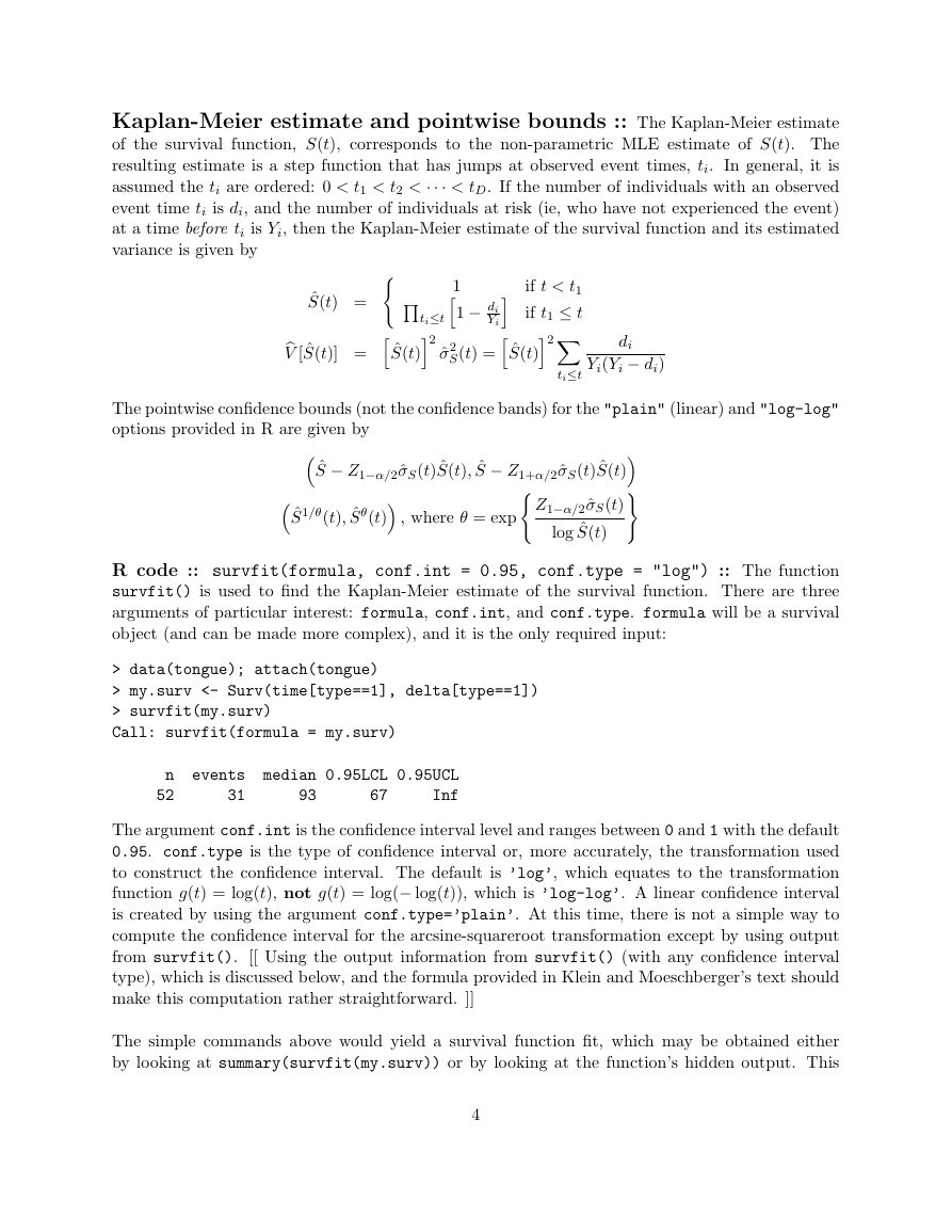
Kaplan-Meier estimate and pointwise bounds :: The Kaplan-Meier estimate
of the survival function, S(t), corresponds to the non-parametric MLE estimate of S(t). The
resulting estimate is a step function that has jumps at observed event times, ti. In general, it is
assumed the ti are ordered: 0 < t1 < t2 < ··· < tD. If the number of individuals with an observed
event time ti is di, and the number of individuals at risk (ie, who have not experienced the event)
at a time before ti is Yi, then the Kaplan-Meier estimate of the survival function and its estimated
variance is given by
i
h ˆS(t)
if t < t1
if t1 ≤ t
i2X
ti≤t
di
Yi(Yi − di)
h
(
Q
h ˆS(t)
i2
ti≤t
1
1 − di
Yi
ˆσ2
S(t) =
ˆS(t) =
bV [ ˆS(t)] =
The pointwise confidence bounds (not the confidence bands) for the "plain" (linear) and "log-log"
options provided in R are given by
ˆS − Z1−α/2ˆσS(t) ˆS(t), ˆS − Z1+α/2ˆσS(t) ˆS(t)
)
ˆS1/θ(t), ˆSθ(t)
, where θ = exp
Z1−α/2ˆσS(t)
(
log ˆS(t)
R code :: survfit(formula, conf.int = 0.95, conf.type = "log") :: The function
survfit() is used to find the Kaplan-Meier estimate of the survival function. There are three
arguments of particular interest: formula, conf.int, and conf.type. formula will be a survival
object (and can be made more complex), and it is the only required input:
> data(tongue); attach(tongue)
> my.surv <- Surv(time[type==1], delta[type==1])
> survfit(my.surv)
Call: survfit(formula = my.surv)
n events
31
52
median 0.95LCL 0.95UCL
Inf
93
67
The argument conf.int is the confidence interval level and ranges between 0 and 1 with the default
0.95. conf.type is the type of confidence interval or, more accurately, the transformation used
to construct the confidence interval. The default is ’log’, which equates to the transformation
function g(t) = log(t), not g(t) = log(− log(t)), which is ’log-log’. A linear confidence interval
is created by using the argument conf.type=’plain’. At this time, there is not a simple way to
compute the confidence interval for the arcsine-squareroot transformation except by using output
from survfit().
[[ Using the output information from survfit() (with any confidence interval
type), which is discussed below, and the formula provided in Klein and Moeschberger’s text should
make this computation rather straightforward. ]]
The simple commands above would yield a survival function fit, which may be obtained either
by looking at summary(survfit(my.surv)) or by looking at the function’s hidden output. This
4
�
hidden information is where the Kaplan-Meier estimate, a 95% confidence bound, along with the
{ti}, {di}, and {Yi} are saved. All of this data will be output by looking at the summary. To get
the output in individual vectors, use the following commands (the actual outputs are omitted for
brevity):
> my.fit <- survfit(my.surv)
> summary(my.fit)$surv
> summary(my.fit)$time
> summary(my.fit)$n.risk
> summary(my.fit)$n.event
> summary(my.fit)$std.err
> summary(my.fit)$lower
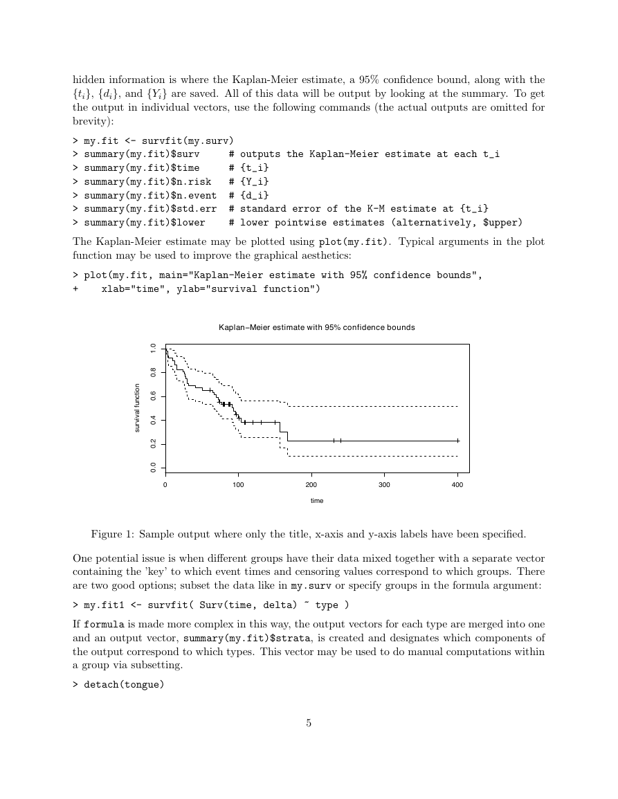
The Kaplan-Meier estimate may be plotted using plot(my.fit). Typical arguments in the plot
function may be used to improve the graphical aesthetics:
# outputs the Kaplan-Meier estimate at each t_i
# {t_i}
# {Y_i}
# {d_i}
# standard error of the K-M estimate at {t_i}
# lower pointwise estimates (alternatively, $upper)
> plot(my.fit, main="Kaplan-Meier estimate with 95% confidence bounds",
+
xlab="time", ylab="survival function")
Figure 1: Sample output where only the title, x-axis and y-axis labels have been specified.
One potential issue is when different groups have their data mixed together with a separate vector
containing the ’key’ to which event times and censoring values correspond to which groups. There
are two good options; subset the data like in my.surv or specify groups in the formula argument:
> my.fit1 <- survfit( Surv(time, delta) ~ type )
If formula is made more complex in this way, the output vectors for each type are merged into one
and an output vector, summary(my.fit)$strata, is created and designates which components of
the output correspond to which types. This vector may be used to do manual computations within
a group via subsetting.
> detach(tongue)
5
01002003004000.00.20.40.60.81.0Kaplan−Meier estimate with 95% confidence boundstimesurvival function�
Confidence bands :: The confidence intervals constructed on the previous pages are only
pointwise confidence intervals. Confidence bands, which are a bit more generalized, can also be
constructed. These bands would be bounds on an entire range of time. That is, for a 95% confidence
band, the probability that any part of the true curve is out of the confidence bands is 0.05. No
functions within the package survival will create confidence bands (in the sense that is being
discussed here), however, a function that will create the bands can be downloaded:
> source(’http://www.stat.ucla.edu/~david/teac/surv/conf-bands.R’)
The form of the function is given as
conf.bands(surv.object, conf.type=’plain’, type=’ep’, tL=NA, tU=NA)
Here, surv.object is a survival object, conf.type may be ’plain’, ’log-log’, or ’asin-sqrt’,
type may be either ’ep’ or ’hall’ (for Hall-Wellner bands), and finally tL and tU are optional
to limit the scope of the confidence bands’ meaning to hold from tL to tU. The appropriate value,
cα(aL, aU ) for EP or kα(aL, aU ) for Hall-Wellner, must be input when requested by conf.bands():
> data(bmt); attach(bmt)
> my.surv <- Surv(t2[group==1], d3[group==1])
> my.cb <- conf.bands(my.surv, type=’hall’, 100, 600)
a_L: 0.1052632
Enter confidence coefficent: 1.3211
a_U: 0.594237
|
> plot(survfit(my.surv), xlim=c(100, 600), xlab=’time’,
+
+
ylab=’Estimated Survival Function’, main=’Reproducing
Confidence Bands for Example 4.2 in Klein/Moeschberger’)
Figure 2: Recall that the default for the pointwise confidence bands is a log transformation, so the
pointwise confidence intervals will not be symmetric.
> lines(my.cb$time, my.cb$lower, lty=3, type=’s’)
> lines(my.cb$time, my.cb$upper, lty=3, type=’s’)
> legend(locator(1), legend=c(’K-M survival estimate’,
+
> detach(bmt)
’pointwise intervals’,’confidence bands’), lty=1:3)
6
1002003004005006000.00.20.40.60.81.0Reproducing Confidence Bands for Example 4.2 in Klein/MoeschbergertimeEstimated Survival FunctionK−M survival estimatepointwise intervalsconfidence bands�
Cumulative Hazard :: The cumulative hazard function and the survival function are
related in the following way for continuous data:
S(t) = exp{−H(t)}
This offers an immediate estimation method of H(t) by taking the negative of the log of ˆS(t):
ˆH(t) = − log ˆS(t). A second method to estimate H(t) is using the Nelson-Aalen estimator and its
variance:
H(t) =X
σ2
di
Y 2
i
ti≤t
˜H(t) =X
ti≤t
(assuming t1 ≤ t, otherwise it is 0),
di
Yi
R code :: There is not a function from survival that will automatically compute either form of
the cumulative hazard function, but this can be done by hand using output from survfit():
> data(tongue); attach(tongue)
> my.surv <- Surv(time[type==1], delta[type==1])
> my.fit <- summary(survfit(my.surv))
> H.hat <- -log(my.fit$surv); H.hat <- c(H.hat, H.hat[length(H.hat)])
Then, using H.hat with my.fit$time, a plot (or table) can be made. Alternatively, the Nelson-
Aalen estimator may be constructed nearly as easily:
> h.sort.of <- my.fit$n.event / my.fit$n.risk
> H.tilde <- vector()
> for(i in 1:length(h.sort.of))
> H.tilde <- c(H.tilde, H.tilde[length(H.tilde)])
> plot(c(my.fit$time, 250), H.hat, xlab=’time’, ylab=’cumulative hazard’,
+
> points(c(my.fit$time, 250), H.tilde, lty=2, type=’s’)
> legend(locator(1), legend=c("H.hat","H.tilde"), lty=1:2)
H.tilde[i] <- sum(h.sort.of[1:i])
main=’comparing cumulative hazards’, ylim=range(c(H.hat, H.tilde)), type=’s’)
Figure 3: Comparing the two cumulative hazard function estimates. 250 was appended to the time
and the hazard functions were extended for aesthetics.
> detach(tongue)
7
�
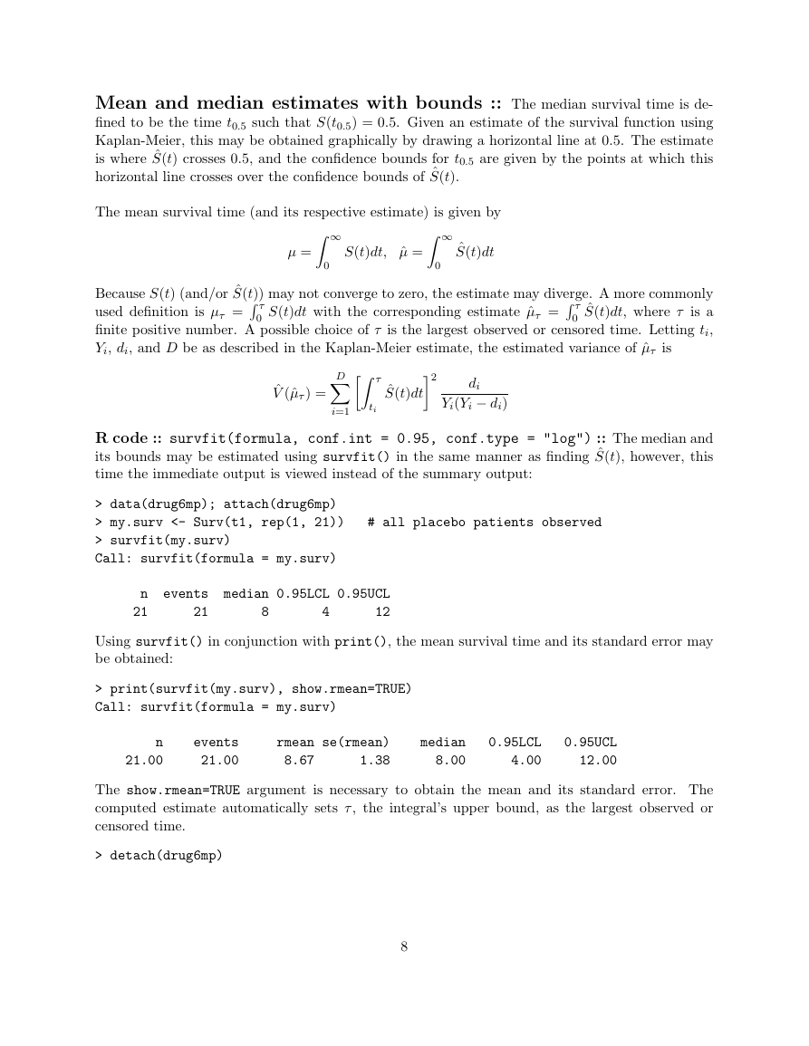
Mean and median estimates with bounds :: The median survival time is de-
fined to be the time t0.5 such that S(t0.5) = 0.5. Given an estimate of the survival function using
Kaplan-Meier, this may be obtained graphically by drawing a horizontal line at 0.5. The estimate
is where ˆS(t) crosses 0.5, and the confidence bounds for t0.5 are given by the points at which this
horizontal line crosses over the confidence bounds of ˆS(t).
The mean survival time (and its respective estimate) is given by
Z ∞
µ =
S(t)dt, ˆµ =
ˆS(t)dt
Z ∞
2
0
used definition is µτ = R τ
Because S(t) (and/or ˆS(t)) may not converge to zero, the estimate may diverge. A more commonly
ˆS(t)dt, where τ is a
finite positive number. A possible choice of τ is the largest observed or censored time. Letting ti,
Yi, di, and D be as described in the Kaplan-Meier estimate, the estimated variance of ˆµτ is
0 S(t)dt with the corresponding estimate ˆµτ = R τ
0
0
Z τ
DX
i=1
ti
ˆV (ˆµτ ) =
ˆS(t)dt
di
Yi(Yi − di)
R code :: survfit(formula, conf.int = 0.95, conf.type = "log") :: The median and
its bounds may be estimated using survfit() in the same manner as finding ˆS(t), however, this
time the immediate output is viewed instead of the summary output:
> data(drug6mp); attach(drug6mp)
> my.surv <- Surv(t1, rep(1, 21))
> survfit(my.surv)
Call: survfit(formula = my.surv)
# all placebo patients observed
n events
21
21
median 0.95LCL 0.95UCL
12
8
4
Using survfit() in conjunction with print(), the mean survival time and its standard error may
be obtained:
> print(survfit(my.surv), show.rmean=TRUE)
Call: survfit(formula = my.surv)
n
21.00
events
21.00
rmean se(rmean)
1.38
8.67
median
8.00
0.95LCL
4.00
0.95UCL
12.00
The show.rmean=TRUE argument is necessary to obtain the mean and its standard error. The
computed estimate automatically sets τ, the integral’s upper bound, as the largest observed or
censored time.
> detach(drug6mp)
8
�






 2023年江西萍乡中考道德与法治真题及答案.doc
 2012年重庆南川中考生物真题及答案.doc
 2013年江西师范大学地理学综合及文艺理论基础考研真题.doc
 2020年四川甘孜小升初语文真题及答案I卷.doc
 2020年注册岩土工程师专业基础考试真题及答案.doc
 2023-2024学年福建省厦门市九年级上学期数学月考试题及答案.doc
 2021-2022学年辽宁省沈阳市大东区九年级上学期语文期末试题及答案.doc
 2022-2023学年北京东城区初三第一学期物理期末试卷及答案.doc
 2018上半年江西教师资格初中地理学科知识与教学能力真题及答案.doc
 2012年河北国家公务员申论考试真题及答案-省级.doc
 2020-2021学年江苏省扬州市江都区邵樊片九年级上学期数学第一次质量检测试题及答案.doc
 2022下半年黑龙江教师资格证中学综合素质真题及答案.doc