498
IEEE TRANSACTIONS ON INFORMATION THEORY, VOL. 47, NO. 2, FEBRUARY 2001
Factor Graphs and the Sum-Product Algorithm
Frank R. Kschischang, Senior Member, IEEE, Brendan J. Frey, Member, IEEE, and
Hans-Andrea Loeliger, Member, IEEE
Abstract—Algorithms that must deal with complicated global
functions of many variables often exploit the manner in which the
given functions factor as a product of “local” functions, each of
which depends on a subset of the variables. Such a factorization
can be visualized with a bipartite graph that we call a factor graph.
In this tutorial paper, we present a generic message-passing algo-
rithm, the sum-product algorithm, that operates in a factor graph.
Following a single, simple computational rule, the sum-product
algorithm computes—either exactly or approximately—var-
ious marginal functions derived from the global function. A
wide variety of algorithms developed in artificial intelligence,
signal processing, and digital communications can be derived as
specific instances of the sum-product algorithm, including the
forward/backward algorithm, the Viterbi algorithm, the iterative
“turbo” decoding algorithm, Pearl’s belief propagation algorithm
for Bayesian networks, the Kalman filter, and certain fast Fourier
transform (FFT) algorithms.
Index Terms—Belief propagation, factor graphs, fast Fourier
transform, forward/backward algorithm, graphical models, iter-
ative decoding, Kalman filtering, marginalization, sum-product
algorithm, Tanner graphs, Viterbi algorithm.
I. INTRODUCTION
T HIS paper provides a tutorial introduction to factor graphs
and the sum-product algorithm, a simple way to under-
stand a large number of seemingly different algorithms that have
been developed in computer science and engineering. We con-
sider algorithms that deal with complicated “global” functions
of many variables and that derive their computational efficiency
by exploiting the way in which the global function factors into
a product of simpler “local” functions, each of which depends
on a subset of the variables. Such a factorization can be visual-
ized using a factor graph, a bipartite graph that expresses which
variables are arguments of which local functions.
Manuscript received August 3, 1998; revised October 17, 2000. The work
of F. R. Kschischang was supported in part, while on leave at the Massachu-
setts Institute of Technology, by the Office of Naval Research under Grant
N00014-96-1-0930, and by the Army Research Laboratory under Cooperative
Agreement DAAL01-96-2-0002. The work of B. J. Frey was supported,
while a Beckman Fellow at the Beckman Institute of Advanced Science and
Technology, University of Illinois at Urbana-Champaign, by a grant from
the Arnold and Mabel Beckman Foundation. The material in this paper was
presented in part at the 35th Annual Allerton Conference on Communication,
Control, and Computing, Monticello, IL, September 1997.
F. R. Kschischang is with the Department of Electrical and Computer
Engineering, University of Toronto, Toronto, ON M5S 3G4, Canada (e-mail:
frank@comm.utoronto.ca).
B. J. Frey is with the Faculty of Computer Science, University of Waterloo,
Waterloo, ON N2L 3G1, Canada, and the Faculty of Electrical and Com-
puter Engineering, University of Illinois at Urbana-Champaign, Urbana, IL
61801-2307 USA (e-mail: frey@.uwaterloo.ca).
H.-A. Loeliger is with the Signal Processing Lab (ISI), ETH Zentrum,
CH-8092 Zürich, Switzerland (e-mail: loeliger@isi.ee.ethz.ch).
Communicated by T. E. Fuja, Associate Editor At Large.
Publisher Item Identifier S 0018-9448(01)00721-0.
The aim of this tutorial paper is to introduce factor graphs
and to describe a generic message-passing algorithm, called the
sum-product algorithm, which operates in a factor graph and at-
tempts to compute various marginal functions associated with
the global function. The basic ideas are very simple; yet, as
we will show, a surprisingly wide variety of algorithms devel-
oped in the artificial intelligence, signal processing, and dig-
ital communications communities may be derived as specific
instances of the sum-product algorithm, operating in an appro-
priately chosen factor graph.
Genealogically, factor graphs are a straightforward gen-
eralization of the “Tanner graphs” of Wiberg et al. [31],
[32]. Tanner [29] introduced bipartite graphs to describe
families of codes which are generalizations of the low-density
parity-check (LDPC) codes of Gallager [11], and also described
the sum-product algorithm in this setting. In Tanner’s original
formulation, all variables are codeword symbols and hence
“visible”; Wiberg et al., introduced “hidden” (latent) state vari-
ables and also suggested applications beyond coding. Factor
graphs take these graph-theoretic models one step further, by
applying them to functions. From the factor-graph perspective
(as we will describe in Section III-A), a Tanner graph for a
code represents a particular factorization of the characteristic
(indicator) function of the code.
While it may seem intuitively reasonable that some algo-
rithms should exploit the manner in which a global function
factors into a product of local functions, the fundamental insight
that many well-known algorithms essentially solve the “MPF”
(marginalize product-of-functions) problem, each in their own
particular setting, was first made explicit in the work of Aji
and McEliece [1]. In a landmark paper [2], Aji and McEliece
develop a “generalized distributive law” (GDL) that in some
cases solves the MPF problem using a “junction tree” represen-
tation of the global function. Factor graphs may be viewed as
an alternative approach with closer ties to Tanner graphs and
previously developed graphical representations for codes. Es-
sentially, every result developed in the junction tree/GDL set-
ting may be translated into an equivalent result in the factor
graph/sum-product algorithm setting, and vice versa. We prefer
the latter setting not only because it is better connected with pre-
vious approaches, but also because we feel that factor graphs are
in some ways easier to describe, giving them a modest pedagog-
ical advantage. Moreover, the sum-product algorithm can often
be applied successfully in situations where exact solutions to the
MPF problem (as provided by junction trees) become computa-
tionally intractable, the most prominent example being the iter-
ative decoding of turbo codes and LDPC codes. In Section VI
we do, however, discuss strategies for achieving exact solutions
to the MPF problem in factor graphs.
0018–9448/01$10.00 © 2001 IEEE
�
KSCHISCHANG et al.: FACTOR GRAPHS AND THE SUM-PRODUCT ALGORITHM
499
There are also close connections between factor graphs and
graphical representations (graphical models) for multidimen-
sional probability distributions such as Markov random fields
[16], [18], [26] and Bayesian (belief) networks [25], [17]. Like
factor graphs, these graphical models encode in their structure a
particular factorization of the joint probability mass function of
several random variables. Pearl’s powerful “belief propagation”
algorithm [25], which operates by “message-passing” in a
Bayesian network, translates immediately into an instance of
the sum-product algorithm operating in a factor graph that
expresses the same factorization. Bayesian networks and belief
propagation have been used previously to explain the iterative
decoding of turbo codes and LDPC codes [9], [10], [19], [21],
[22], [24],
the most powerful practically decodable codes
known. Note, however, that Wiberg [31] had earlier described
these decoding algorithms as instances of the sum-product
algorithm; see also [7].
We begin the paper in Section II with a small worked example
that illustrates the operation of the sum-product algorithm in a
simple factor graph. We will see that when a factor graph is
cycle-free, then the structure of the factor graph not only en-
codes the way in which a given function factors, but also en-
codes expressions for computing the various marginal functions
associated with the given function. These expressions lead di-
rectly to the sum-product algorithm.
In Section III, we show how factor graphs may be used as a
system and signal-modeling tool. We see that factor graphs are
compatible both with “behavioral” and “probabilistic” modeling
styles. Connections between factor graphs and other graphical
models are described briefly in Appendix B, where we recover
Pearl’s belief propagation algorithm as an instance of the sum-
product algorithm.
In Section IV, we apply the sum-product algorithm to
trellis-structured (hidden Markov) models, and obtain the
forward/backward algorithm, the Viterbi algorithm, and the
Kalman filter as instances of the sum-product algorithm. In
Section V, we consider factor graphs with cycles, and obtain
the iterative algorithms used to decode turbo-like codes as
instances of the sum-product algorithm.
In Section VI, we describe several generic transformations
by which a factor graph with cycles may sometimes be con-
verted—often at great expense in complexity—to an equivalent
cycle-free form. We apply these ideas to the factor graph repre-
senting the discrete Fourier transform (DFT) kernel, and derive
a fast Fourier transform (FFT) algorithm as an instance of the
sum-product algorithm.
Some concluding remarks are given in Section VII.
II. MARGINAL FUNCTIONS, FACTOR GRAPHS, AND THE
SUM-PRODUCT ALGORITHM
,
Throughout this paper we deal with functions of many vari-
be a collection of variables, in which,
takes on values in some (usually finite) domain
-valued function
ables. Let
for each ,
(or alphabet)
of these variables, i.e., a function with domain
be an
. Let
of
. The domain
and codomain
is called the configuration
space for the given collection of variables, and each element of
is a particular configuration of the variables, i.e., an assign-
of may in
ment of a value to each variable. The codomain
general be any semiring [2], [31, Sec. 3.6]; however, at least ini-
is the
tially, we will lose nothing essential by assuming that
set of real numbers.
Assuming that summation in
ated with every function
. For each
tions
summing the value of
the variables that have
.
is well defined, then associ-
are marginal func-
is obtained by
over all configurations of
, the value of
This type of sum is so central to this paper that we introduce
a nonstandard notation to handle it: the “not-sum” or summary.
Instead of indicating the variables being summed over, we indi-
is
cate those variables not being summed over. For example, if
, then the “summary
a function of three variables
for
” is denoted by
, and
,
In this notation we have
i.e., the th marginal function associated with
the summary for
of
.
is
We are interested in developing efficient procedures for com-
puting marginal functions that a) exploit the way in which the
global function factors, using the distributive law to simplify the
summations, and b) reuses intermediate values (partial sums).
As we will see, such procedures can be expressed very natu-
rally by use of a factor graph.
Suppose that
local functions, each having some subset of
arguments; i.e., suppose that
factors into a product of several
as
(1)
is a discrete index set,
is a subset of
is a function having the elements of
,
as argu-
where
and
ments.
Definition: A factor graph is a bipartite graph that expresses
the structure of the factorization (1). A factor graph has a vari-
, a factor node for each local func-
able node for each variable
to factor node
tion
, and an edge-connecting variable node
if and only if
is an argument of
.
A factor graph is thus a standard bipartite graphical represen-
tation of a mathematical relation—in this case, the “is an argu-
ment of” relation between variables and local functions.
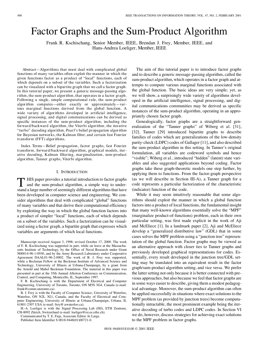
Example 1 (A Simple Factor Graph): Let
be a function of five variables, and suppose that
can
be expressed as a product
(2)
�
500
IEEE TRANSACTIONS ON INFORMATION THEORY, VOL. 47, NO. 2, FEBRUARY 2001
Fig. 1. A factor graph for the product f (x )f (x )f (x ; x ; x )
� f (x ; x )f (x ; x ).
of five factors, so that
,
,
,
, and
,
. The factor graph that corresponds to (2) is shown in
Fig. 1.
A. Expression Trees
In many situations (for example, when
rep-
resents a joint probability mass function), we are interested in
. We can obtain an ex-
computing the marginal functions
pression for each marginal function by using (2) and exploiting
the distributive law.
To illustrate, we write
from Example 1 as
or, in summary notation
Similarly, we find that
(3)
(4)
In computer
science, arithmetic expressions
like the
right-hand sides of (3) and (4) are often represented by or-
dered rooted trees [28, Sec. 8.3], here called expression trees,
in which internal vertices (i.e., vertices with descendants)
represent arithmetic operators (e.g., addition, multiplication,
negation, etc.) and leaf vertices (i.e., vertices without descen-
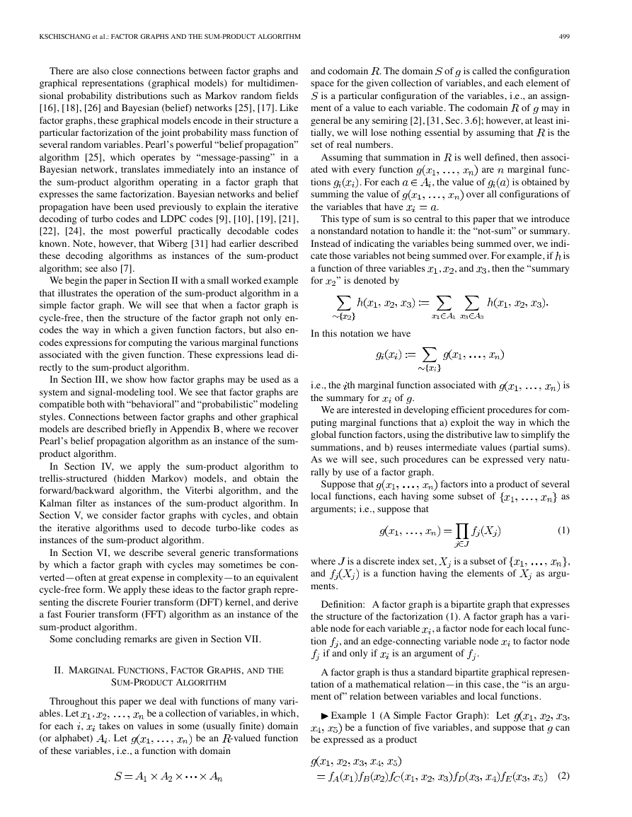
dants) represent variables or constants. For example, the tree of
. When the operators
Fig. 2 represents the expression
in an expression tree are restricted to those that are completely
symmetric in their operands (e.g., multiplication and addition),
Fig. 2. An expression tree representing x(y + z).
it is unnecessary to order the vertices to avoid ambiguity in
interpreting the expression represented by the tree.
In this paper, we extend expression trees so that the leaf ver-
tices represent functions, not just variables or constants. Sums
and products in such expression trees combine their operands in
the usual (pointwise) manner in which functions are added and
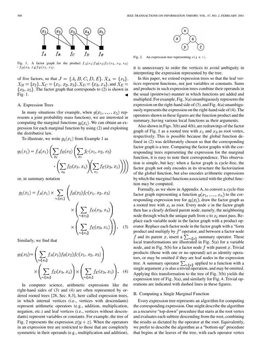
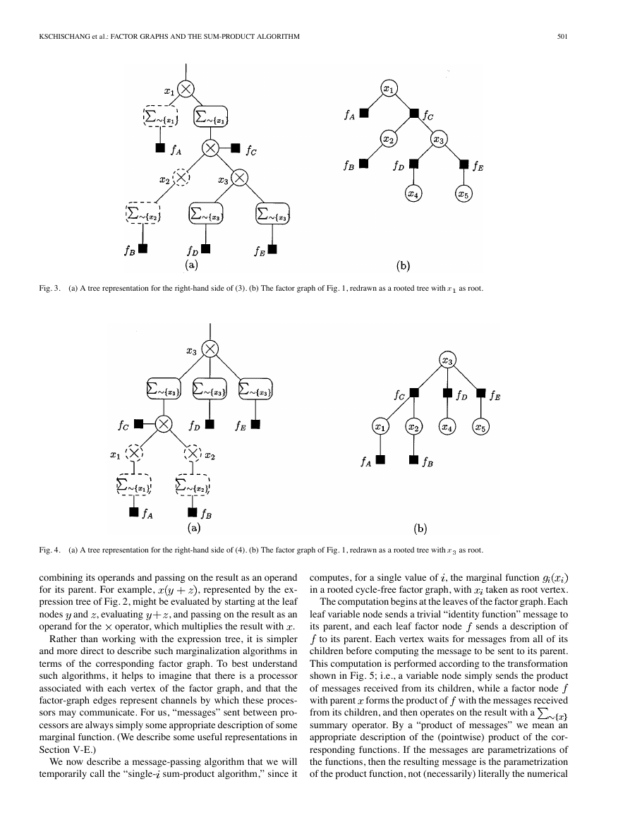
multiplied. For example, Fig. 3(a) unambiguously represents the
expression on the right-hand side of (3), and Fig. 4(a) unambigu-
ously represents the expression on the right-hand side of (4). The
operators shown in these figures are the function product and the
summary, having various local functions as their arguments.
and
Also shown in Figs. 3(b) and 4(b), are redrawings of the factor
as root vertex,
graph of Fig. 1 as a rooted tree with
respectively. This is possible because the global function de-
fined in (2) was deliberately chosen so that the corresponding
factor graph is a tree. Comparing the factor graphs with the cor-
responding trees representing the expression for the marginal
function, it is easy to note their correspondence. This observa-
tion is simple, but key: when a factor graph is cycle-free, the
factor graph not only encodes in its structure the factorization
of the global function, but also encodes arithmetic expressions
by which the marginal functions associated with the global func-
tion may be computed.
as root. Every node
Formally, as we show in Appendix A, to convert a cycle-free
to the cor-
factor graph representing a function
, draw the factor graph as
responding expression tree for
in the factor graph
a rooted tree with
then has a clearly defined parent node, namely, the neighboring
node through which the unique path from to must pass. Re-
place each variable node in the factor graph with a product op-
erator. Replace each factor node in the factor graph with a “form
product and multiply by ” operator, and between a factor node
summary operator. These
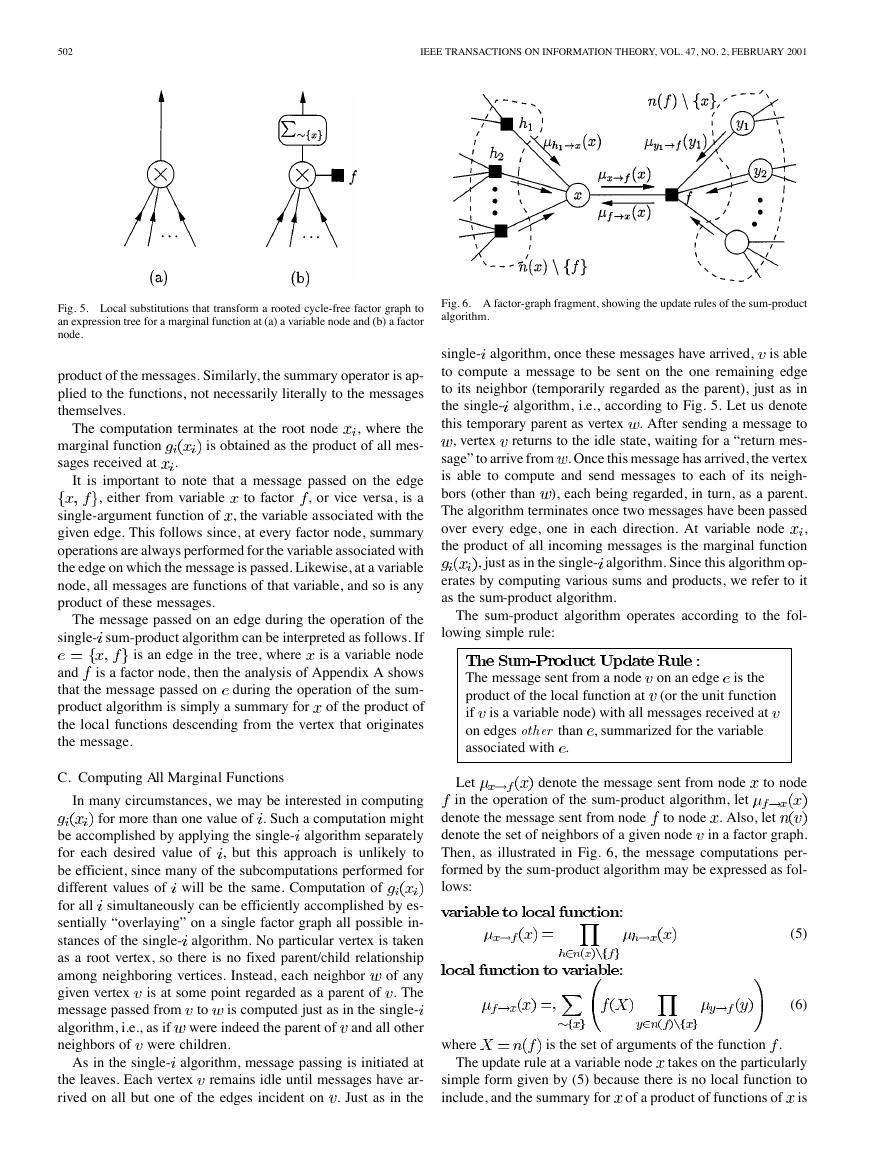
local transformations are illustrated in Fig. 5(a) for a variable
node, and in Fig. 5(b) for a factor node with parent
. Trivial
products (those with one or no operand) act as identity opera-
tors, or may be omitted if they are leaf nodes in the expression
applied to a function with a
tree. A summary operator
is also a trivial operation, and may be omitted.
single argument
Applying this transformation to the tree of Fig. 3(b) yields the
expression tree of Fig. 3(a), and similarly for Fig. 4. Trivial op-
erations are indicated with dashed lines in these figures.
and its parent
, insert a
B. Computing a Single Marginal Function
Every expression tree represents an algorithm for computing
the corresponding expression. One might describe the algorithm
as a recursive “top-down” procedure that starts at the root vertex
and evaluates each subtree descending from the root, combining
the results as dictated by the operator at the root. Equivalently,
we prefer to describe the algorithm as a “bottom-up” procedure
that begins at the leaves of the tree, with each operator vertex
�
KSCHISCHANG et al.: FACTOR GRAPHS AND THE SUM-PRODUCT ALGORITHM
501
Fig. 3.
(a) A tree representation for the right-hand side of (3). (b) The factor graph of Fig. 1, redrawn as a rooted tree with x as root.
Fig. 4.
(a) A tree representation for the right-hand side of (4). (b) The factor graph of Fig. 1, redrawn as a rooted tree with x as root.
and , evaluating
combining its operands and passing on the result as an operand
, represented by the ex-
for its parent. For example,
pression tree of Fig. 2, might be evaluated by starting at the leaf
, and passing on the result as an
nodes
operator, which multiplies the result with .
operand for the
Rather than working with the expression tree, it is simpler
and more direct to describe such marginalization algorithms in
terms of the corresponding factor graph. To best understand
such algorithms, it helps to imagine that there is a processor
associated with each vertex of the factor graph, and that the
factor-graph edges represent channels by which these proces-
sors may communicate. For us, “messages” sent between pro-
cessors are always simply some appropriate description of some
marginal function. (We describe some useful representations in
Section V-E.)
We now describe a message-passing algorithm that we will
temporarily call the “single- sum-product algorithm,” since it
computes, for a single value of , the marginal function
in a rooted cycle-free factor graph, with
taken as root vertex.
The computation begins at the leaves of the factor graph. Each
leaf variable node sends a trivial “identity function” message to
sends a description of
its parent, and each leaf factor node
to its parent. Each vertex waits for messages from all of its
children before computing the message to be sent to its parent.
This computation is performed according to the transformation
shown in Fig. 5; i.e., a variable node simply sends the product
of messages received from its children, while a factor node
with parent
from its children, and then operates on the result with a
summary operator. By a “product of messages” we mean an
appropriate description of the (pointwise) product of the cor-
responding functions. If the messages are parametrizations of
the functions, then the resulting message is the parametrization
of the product function, not (necessarily) literally the numerical
forms the product of with the messages received
�
502
IEEE TRANSACTIONS ON INFORMATION THEORY, VOL. 47, NO. 2, FEBRUARY 2001
Fig. 5. Local substitutions that transform a rooted cycle-free factor graph to
an expression tree for a marginal function at (a) a variable node and (b) a factor
node.
product of the messages. Similarly, the summary operator is ap-
plied to the functions, not necessarily literally to the messages
themselves.
The computation terminates at the root node
, where the
is obtained as the product of all mes-
marginal function
sages received at
.
to factor
It is important to note that a message passed on the edge
, or vice versa, is a
, either from variable
, the variable associated with the
single-argument function of
given edge. This follows since, at every factor node, summary
operations are always performed for the variable associated with
the edge on which the message is passed. Likewise, at a variable
node, all messages are functions of that variable, and so is any
product of these messages.
is an edge in the tree, where
The message passed on an edge during the operation of the
single- sum-product algorithm can be interpreted as follows. If
is a variable node
is a factor node, then the analysis of Appendix A shows
and
during the operation of the sum-
that the message passed on
of the product of
product algorithm is simply a summary for
the local functions descending from the vertex that originates
the message.
C. Computing All Marginal Functions
In many circumstances, we may be interested in computing
for more than one value of . Such a computation might
be accomplished by applying the single- algorithm separately
, but this approach is unlikely to
for each desired value of
be efficient, since many of the subcomputations performed for
different values of will be the same. Computation of
for all
simultaneously can be efficiently accomplished by es-
sentially “overlaying” on a single factor graph all possible in-
stances of the single- algorithm. No particular vertex is taken
as a root vertex, so there is no fixed parent/child relationship
of any
among neighboring vertices. Instead, each neighbor
. The
given vertex
is computed just as in the single-
message passed from to
algorithm, i.e., as if were indeed the parent of
and all other
neighbors of were children.
is at some point regarded as a parent of
As in the single- algorithm, message passing is initiated at
remains idle until messages have ar-
the leaves. Each vertex
rived on all but one of the edges incident on . Just as in the
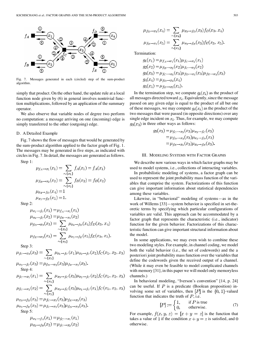
Fig. 6. A factor-graph fragment, showing the update rules of the sum-product
algorithm.
, vertex
single- algorithm, once these messages have arrived,
is able
to compute a message to be sent on the one remaining edge
to its neighbor (temporarily regarded as the parent), just as in
the single- algorithm, i.e., according to Fig. 5. Let us denote
. After sending a message to
this temporary parent as vertex
returns to the idle state, waiting for a “return mes-
sage” to arrive from . Once this message has arrived, the vertex
is able to compute and send messages to each of its neigh-
), each being regarded, in turn, as a parent.
bors (other than
The algorithm terminates once two messages have been passed
,
over every edge, one in each direction. At variable node
the product of all incoming messages is the marginal function
, just as in the single- algorithm. Since this algorithm op-
erates by computing various sums and products, we refer to it
as the sum-product algorithm.
The sum-product algorithm operates according to the fol-
lowing simple rule:
The message sent from a node
product of the local function at
is a variable node) with all messages received at
if
on edges other than , summarized for the variable
associated with .
on an edge
(or the unit function
is the
Let
denote the message sent from node
in the operation of the sum-product algorithm, let
to node
denote the message sent from node
denote the set of neighbors of a given node
in a factor graph.
Then, as illustrated in Fig. 6, the message computations per-
formed by the sum-product algorithm may be expressed as fol-
lows:
to node . Also, let
(5)
(6)
where
is the set of arguments of the function .
The update rule at a variable node
takes on the particularly
simple form given by (5) because there is no local function to
is
include, and the summary for
of a product of functions of
�
KSCHISCHANG et al.: FACTOR GRAPHS AND THE SUM-PRODUCT ALGORITHM
503
Termination:
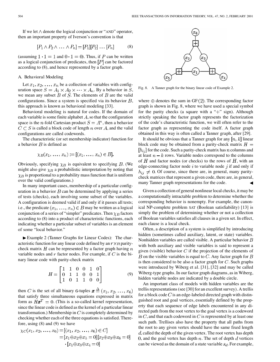
Fig. 7. Messages generated in each (circled) step of the sum-product
algorithm.
simply that product. On the other hand, the update rule at a local
function node given by (6) in general involves nontrivial func-
tion multiplications, followed by an application of the summary
operator.
We also observe that variable nodes of degree two perform
no computation: a message arriving on one (incoming) edge is
simply transferred to the other (outgoing) edge.
In the termination step, we compute
as the product of
. Equivalently, since the message
all messages directed toward
passed on any given edge is equal to the product of all but one
as the product of the
of these messages, we may compute
two messages that were passed (in opposite directions) over any
. Thus, for example, we may compute
single edge incident on
in three other ways as follows:
D. A Detailed Example
Fig. 7 shows the flow of messages that would be generated by
the sum-product algorithm applied to the factor graph of Fig. 1.
The messages may be generated in five steps, as indicated with
circles in Fig. 7. In detail, the messages are generated as follows.
Step 1:
Step 2:
Step 3:
Step 4:
Step 5:
III. MODELING SYSTEMS WITH FACTOR GRAPHS
We describe now various ways in which factor graphs may be
used to model systems, i.e., collections of interacting variables.
In probabilistic modeling of systems, a factor graph can be
used to represent the joint probability mass function of the vari-
ables that comprise the system. Factorizations of this function
can give important information about statistical dependencies
among these variables.
Likewise, in “behavioral” modeling of systems—as in the
work of Willems [33]—system behavior is specified in set-the-
oretic terms by specifying which particular configurations of
variables are valid. This approach can be accommodated by a
factor graph that represents the characteristic (i.e., indicator)
function for the given behavior. Factorizations of this charac-
teristic function can give important structural information about
the model.
In some applications, we may even wish to combine these
two modeling styles. For example, in channel coding, we model
both the valid behavior (i.e., the set of codewords) and the a
posteriori joint probability mass function over the variables that
define the codewords given the received output of a channel.
(While it may even be feasible to model complicated channels
with memory [31], in this paper we will model only memoryless
channels.)
In behavioral modeling, “Iverson’s convention” [14, p. 24]
is a predicate (Boolean proposition) in-
-valued
can be useful. If
volving some set of variables, then
function that indicates the truth of
is the
, i.e.
For example,
takes a value of
otherwise.
if the condition
if
is true
otherwise.
(7)
is the function that
is satisfied, and
�
504
IEEE TRANSACTIONS ON INFORMATION THEORY, VOL. 47, NO. 2, FEBRUARY 2001
If we let
denote the logical conjunction or “AND” operator,
then an important property of Iverson’s convention is that
(8)
(assuming
as a logical conjunction of predicates, then
according to (8), and hence represented by a factor graph.
can be written
can be factored
). Thus, if
and
A. Behavioral Modeling
Let
uration space
we mean any subset
configurations. Since a system is specified via its behavior
this approach is known as behavioral modeling [33].
be a collection of variables with config-
. By a behavior in ,
are the valid
,
. The elements of
of
each variable is some finite alphabet
space is the -fold Cartesian product
Behavioral modeling is natural for codes. If the domain of
, so that the configuration
, then a behavior
, and the valid
is called a block code of length
over
configurations are called codewords.
The characteristic (or set membership indicator) function for
Fig. 8. A Tanner graph for the binary linear code of Example 2.
denotes the sum in GF
where
. The corresponding factor
graph is shown in Fig. 8, where we have used a special symbol
for the parity checks (a square with a “ ” sign). Although
strictly speaking the factor graph represents the factorization
of the code’s characteristic function, we will often refer to the
factor graph as representing the code itself. A factor graph
obtained in this way is often called a Tanner graph, after [29].
linear
It should be obvious that a Tanner graph for any
a behavior
is defined as
block code may be obtained from a parity-check matrix
Obviously, specifying
might also give
. (We
a probabilistic interpretation by noting that
is proportional to a probability mass function that is uniform
is equivalent to specifying
over the valid configurations.)
In many important cases, membership of a particular config-
can be determined by applying a series
uration in a behavior
of tests (checks), each involving some subset of the variables.
A configuration is deemed valid if and only if it passes all tests;
may be written as a logical
i.e., the predicate
factors
conjunction of a series of “simpler” predicates. Then
according to (8) into a product of characteristic functions, each
indicating whether a particular subset of variables is an element
of some “local behavior.”
Example 2 (Tanner Graphs for Linear Codes): The char-
parity-
acteristic function for any linear code defined by an
check matrix
variable nodes and
nary linear code with parity-check matrix
factor nodes. For example, if
can be represented by a factor graph having
is the bi-
(9)
is the set of all binary -tuples
then
that satisfy three simultaneous equations expressed in matrix
. (This is a so-called kernel representation,
form as
since the linear code is defined as the kernel of a particular linear
is completely determined by
transformation.) Membership in
checking whether each of the three equations is satisfied. There-
fore, using (8) and (9) we have
for the code. Such a parity-check matrix has
and factor nodes (or checks) to the rows of
at least
of
edge-connecting factor node
columns and
rows. Variable nodes correspond to the columns
, with an
if and only if
. Of course, since there are, in general, many parity-
check matrices that represent a given code, there are, in general,
many Tanner graph representations for the code.
to variable node
Given a collection of general nonlinear local checks, it may be
a computationally intractable problem to determine whether the
corresponding behavior is nonempty. For example, the canon-
ical NP-complete problem SAT (Boolean satisfiability) [13] is
simply the problem of determining whether or not a collection
of Boolean variables satisfies all clauses in a given set. In effect,
each clause is a local check.
Often, a description of a system is simplified by introducing
hidden (sometimes called auxiliary, latent, or state) variables.
Nonhidden variables are called visible. A particular behavior
with both auxiliary and visible variables is said to represent a
if the projection of the elements of
given (visible) behavior
on the visible variables is equal to
. Any factor graph for
is then considered to be also a factor graph for
. Such graphs
were introduced by Wiberg et al. [31], [32] and may be called
Wiberg-type graphs. In our factor graph diagrams, as in Wiberg,
hidden variable nodes are indicated by a double circle.
An important class of models with hidden variables are the
trellis representations (see [30] for an excellent survey). A trellis
is an edge-labeled directed graph with distin-
for a block code
guished root and goal vertices, essentially defined by the prop-
erty that each sequence of edge labels encountered in any di-
rected path from the root vertex to the goal vertex is a codeword
is represented by at least one
in
such path. Trellises also have the property that all paths from
the root to any given vertex should have the same fixed length
, called the depth of the given vertex. The root vertex has depth
, and the goal vertex has depth . The set of depth
vertices
. For example,
can be viewed as the domain of a state variable
, and that each codeword in
�
KSCHISCHANG et al.: FACTOR GRAPHS AND THE SUM-PRODUCT ALGORITHM
505
Fig. 9.
(a) A trellis and (b) the corresponding Wiberg-type graph for the code of Fig. 8.
Fig. 9(a) is a trellis for the code of Example 2. Vertices at the
same depth are grouped vertically. The root vertex is leftmost,
the goal vertex is rightmost, and edges are implicitly directed
from left to right.
A trellis divides naturally into
sections, where the th trellis
is the subgraph of the trellis induced by the vertices
and depth . The set of edge labels in may be
. In effect, each
defines a “local behavior” that constrains the
section
at depth
viewed as the domain of a (visible) variable
trellis section
possible combinations of
, and
,
.
Globally, a trellis defines a behavior in the configuration
. A configu-
space of the variables
ration of these variables is valid if and only if it satisfies the
local constraints imposed by each of the trellis sections. The
characteristic function for this behavior thus factors naturally
factors, where the th factor corresponds to the th trellis
into
section
as its arguments.
and has
, and
,
The following example illustrates these concepts in detail for
the code of Example 2.
Example 3 (A Trellis Description): Fig. 9(a) shows a
trellis for the code of Example 2, and Fig. 9(b) shows the
corresponding Wiberg-type graph. In addition to the visible
, there are also hidden (state)
variable nodes
. Each local check, shown as a
variable nodes
generic factor node (black square), corresponds to one section
of the trellis.
In this example, the local behavior
corresponding to the
second trellis section from the left in Fig. 9 consists of the fol-
lowing triples
:
(10)
are taken to
where the domains of the state variables
, respectively, numbered from bottom
be
to top in Fig. 9(a). Each element of the local behavior corre-
sponds to one trellis edge. The corresponding factor node in
the Wiberg-type graph is the indicator function
and
and
.
It is important to note that a factor graph corresponding to
a trellis is cycle-free. Since every code has a trellis representa-
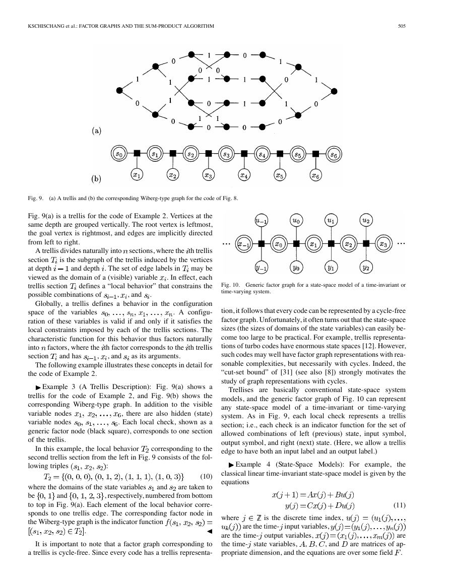
Fig. 10. Generic factor graph for a state-space model of a time-invariant or
time-varying system.
tion, it follows that every code can be represented by a cycle-free
factor graph. Unfortunately, it often turns out that the state-space
sizes (the sizes of domains of the state variables) can easily be-
come too large to be practical. For example, trellis representa-
tions of turbo codes have enormous state spaces [12]. However,
such codes may well have factor graph representations with rea-
sonable complexities, but necessarily with cycles. Indeed, the
“cut-set bound” of [31] (see also [8]) strongly motivates the
study of graph representations with cycles.
Trellises are basically conventional state-space system
models, and the generic factor graph of Fig. 10 can represent
any state-space model of a time-invariant or time-varying
system. As in Fig. 9, each local check represents a trellis
section; i.e., each check is an indicator function for the set of
allowed combinations of left (previous) state, input symbol,
output symbol, and right (next) state. (Here, we allow a trellis
edge to have both an input label and an output label.)
Example 4 (State-Space Models): For example,
the
classical linear time-invariant state-space model is given by the
equations
where
is the discrete time index,
are the time-
input variables,
(11)
are the time- output variables,
the time-
propriate dimension, and the equations are over some field
are
are matrices of ap-
.
state variables,
, and
,
,
�


 2023年江西萍乡中考道德与法治真题及答案.doc
 2012年重庆南川中考生物真题及答案.doc
 2013年江西师范大学地理学综合及文艺理论基础考研真题.doc
 2020年四川甘孜小升初语文真题及答案I卷.doc
 2020年注册岩土工程师专业基础考试真题及答案.doc
 2023-2024学年福建省厦门市九年级上学期数学月考试题及答案.doc
 2021-2022学年辽宁省沈阳市大东区九年级上学期语文期末试题及答案.doc
 2022-2023学年北京东城区初三第一学期物理期末试卷及答案.doc
 2018上半年江西教师资格初中地理学科知识与教学能力真题及答案.doc
 2012年河北国家公务员申论考试真题及答案-省级.doc
 2020-2021学年江苏省扬州市江都区邵樊片九年级上学期数学第一次质量检测试题及答案.doc
 2022下半年黑龙江教师资格证中学综合素质真题及答案.doc