张量子空间算法.pdf

发布时间：2022-06-14 发布人：admin 分类：说明书资料大小：0.54M 资料格式：pdf 举报版权申诉

5644682a-3fc1-48be-82f0-31d3f75b3978.pdf-第1页.png

第1页 / 共10页

5644682a-3fc1-48be-82f0-31d3f75b3978.pdf-第2页.png

第2页 / 共10页

5644682a-3fc1-48be-82f0-31d3f75b3978.pdf-第3页.png

第3页 / 共10页

5644682a-3fc1-48be-82f0-31d3f75b3978.pdf-第4页.png

第4页 / 共10页

5644682a-3fc1-48be-82f0-31d3f75b3978.pdf-第5页.png

第5页 / 共10页

5644682a-3fc1-48be-82f0-31d3f75b3978.pdf-第6页.png

第6页 / 共10页

5644682a-3fc1-48be-82f0-31d3f75b3978.pdf-第7页.png

第7页 / 共10页

5644682a-3fc1-48be-82f0-31d3f75b3978.pdf-第8页.png

第8页 / 共10页

Introduction

Background

Principal Component Analysis

Multilinear Analysis

Problem Definition

Tensor Analysis

Offline Tensor Analysis

Dynamic Tensor Analysis

Streaming Tensor Analysis

Applications

Anomaly Detection

Multi-way Latent Semantic Indexing

Experiments

Datasets

Efficiency Evaluation

Data mining case studies

Anomaly Detection

Multi-way LSI

Related Work

Conclusions

Acknowledgement

REFERENCES -9pt

Beyond Streams and Graphs: Dynamic Tensor Analysis Jimeng Sun† Dacheng Tao‡ Christos Faloutsos † † Computer Science Department, Carnegie Mellon University, Pittsburgh,USA ‡ School of Computer Science and Information Systems, Birkbeck College, University of London,UK {jimeng,christos}@cs.cmu.edu, dacheng@dcs.bbk.ac.uk ABSTRACT How do we ﬁnd patterns in author-keyword associations, evolving over time? Or in DataCubes, with product-branch- customer sales information? Matrix decompositions, like principal component analysis (PCA) and variants, are in- valuable tools for mining, dimensionality reduction, feature selection, rule identiﬁcation in numerous settings like stream- ing data, text, graphs, social networks and many more. However, they have only two orders, like author and key- word, in the above example. We propose to envision such higher order data as tensors, and tap the vast literature on the topic. However, these methods do not necessarily scale up, let alone operate on semi-inﬁnite streams. Thus, we introduce the dynamic ten- sor analysis (DTA) method, and its variants. DTA provides a compact summary for high-order and high-dimensional data, and it also reveals the hidden correlations. Algorith- mically, we designed DTA very carefully so that it is (a) scalable, (b) space eﬃcient (it does not need to store the past) and (c) fully automatic with no need for user deﬁned parameters. Moreover, we propose STA, a streaming tensor analysis method, which provides a fast, streaming approxi- mation to DTA. We implemented all our methods, and applied them in two real settings, namely, anomaly detection and multi-way latent semantic indexing. We used two real, large datasets, one on network ﬂow data (100GB over 1 month) and one from DBLP (200MB over 25 years). Our experiments show that our methods are fast, accurate and that they ﬁnd in- teresting patterns and outliers on the real datasets. 1. INTRODUCTION Given a keyword-author-timestamp-conference bibliogra- phy, how can we ﬁnd patterns and latent concepts? Given Internet traﬃc data (who sends packets to whom, on what port, and when), how can we ﬁnd anomalies, patterns and summaries? Anomalies could be, e.g., port-scanners, pat- terns could be of the form “workstations are down on week- Permission to make digital or hard copies of all or part of this work for personal or classroom use is granted without fee provided that copies are not made or distributed for proﬁt or commercial advantage and that copies bear this notice and the full citation on the ﬁrst page. To copy otherwise, to republish, to post on servers or to redistribute to lists, requires prior speciﬁc permission and/or a fee. KDD’06, August 20–23, 2006, Philadelphia, Pennsylvania, USA. Copyright 2006 ACM 1-59593-339-5/06/0008 ...$5.00. ends, while servers spike at Fridays for backups”. Sum- maries like the one above are useful to give us an idea what is the past (which is probably the norm), so that we can spot deviations from it in the future. Matrices and matrix operations like SVD/PCA have played a vital role in ﬁnding patterns when the dataset is “2-dimensional”, and can thus be represented as a matrix. Important appli- cations of this view point include numerous settings like: 1) information retrieval, where the data can be turned into a document-term matrix, and then apply LSI [9, 24]; 2) market basket analysis, with customer-products ma- trices, where we can apply association rules [2] or “Ratio Rules” [21]; 3) the web, where both rows and columns are pages, and links correspond to edges between them; then we can apply HITS [19] or pageRank [3] to ﬁnd hubs, au- thorities and inﬂuential nodes; all of them are identical or closely related to eigen analysis or derivatives; 4) social networks, and in fact, any graph (with un-labelled edges): people are rows and columns; edges again correspond to non- zero entries in the adjacency matrix. The network value of a customer [13] has close ties to the ﬁrst eigenvector; graph partitioning [18] is often done through matrix alge- bra (e.g. spectral clustering [16]); 5) streams and co- evolving sequences can also be envisioned as matrices: each data source (sensor) corresponds to a row, and each time-tick to a column. Then we can do multivariate anal- ysis or SVD [25],“sketches” and random projections [14] to ﬁnd patterns and outliers. The need for tensors: Powerful as they may be, matrix- based tools can handle neither of the two problems we stated in the beginning. The crux is that matrices have only two “dimensions” (e.g., “customers” and “products”), while we may often need more, like “authors”, “keywords”, “times- tamps”, “conferences”. This is exactly what a tensor is, and of course, a tensor is a generalization of a matrix (and of a vector, and of a scalar). We propose to envision all such problems as tensor problems, to use the vast literature of tensors to our beneﬁt, and to introduce new tensor analysis tools, tailored for streaming applications. Using tensors, we OLAP dimensionality dimension attribute value this paper order mode dimension tensor literature order/mode order/mode dimension Table 1: Terminology correspondence can attack an even wider range of problems, that matrices can not even touch. For example, 1) Rich, time-evolving net- work traﬃc data, as mentioned earlier: we have tensors of

order M = 3, with modes “source-IP”, “destination-IP” and “port” over time. 2) Labeled graphs and social networks: suppose that we have diﬀerent types of edges in a social net- work (eg., who-called-whom, who-likes-whom, who-emailed- whom, who-borrowed-money-from-whom). In that case, we have a 3rd order tensor, with edge-type being the 3rd mode. Over time, we have multiple 3rd order tensors, which are still within the reach of our upcoming tools. 3) Microarray data, with gene expressions evolving over time [32]. Here we have genes-proteins over time, and we record the expression level: a series of 2nd order tensors. 4) All OLAP and Dat- aCube applications: customer-product-branch sales data is a 3rd order tensor; and so is patient-diagnoses-drug treat- ment data. Motivating example: Let us consider the network mon- itoring example. Here we have network ﬂows arriving very fast and continuously through routers, where each ﬂow con- sists of source IP, destination IP, port number and the num- ber of packets. How to monitor the dynamic traﬃc behav- ior? How to identify anomalies which can signify a potential intrusion, or worm propagation, or an attack? What are the correlations across the various sources, destinations and ports? Ports Sources DTA/STA n o i t a n i t s e D n o i t c e o r P j Projection Port Core Tensor Source Projection i t a n s n o i t s e D Description a vector (lower-case bold) the i-element of vector v a matrix (upper-case bold) the transpose of A a sequence of N matrices A1, . . . , An the entry (i, j) of A Symbol v v(i) A AT Ai|n i=1 A(i, j) A(i, :) or A(:, i) i-th row or column of A A A(i1, . . . , iM ) M Ni a tensor (calligraphic style) the element of X with index (i1, . . . , iM ) the order of the tensor the dimensionality of the ith mode (1 ≤ i ≤ M ) Table 2: Description of notation. • Systematic evaluation on large, real datasets, where our tools found patterns and anomalies, and provided large speed-ups over competitors. The rest of the paper is organized as the following: Section 2 introduces the necessary background. Then Section 3 for- mally deﬁnes the problem and gives an overview of the methods. Section 4 presents the key methods, dynamic ten- sor analysis (DTA) and streaming tensor analysis (STA). Using DTA or STA, Section 5 illustrates two important ap- plications: anomaly detection and multi-way latent seman- tics indexing. In Section 6 and Section 7 we extensively evaluate all the proposed methods using two real datasets. Section 8 discusses the related work. Finally we conclude in Section 9. (a) original Tensor (b) DTA result 2. 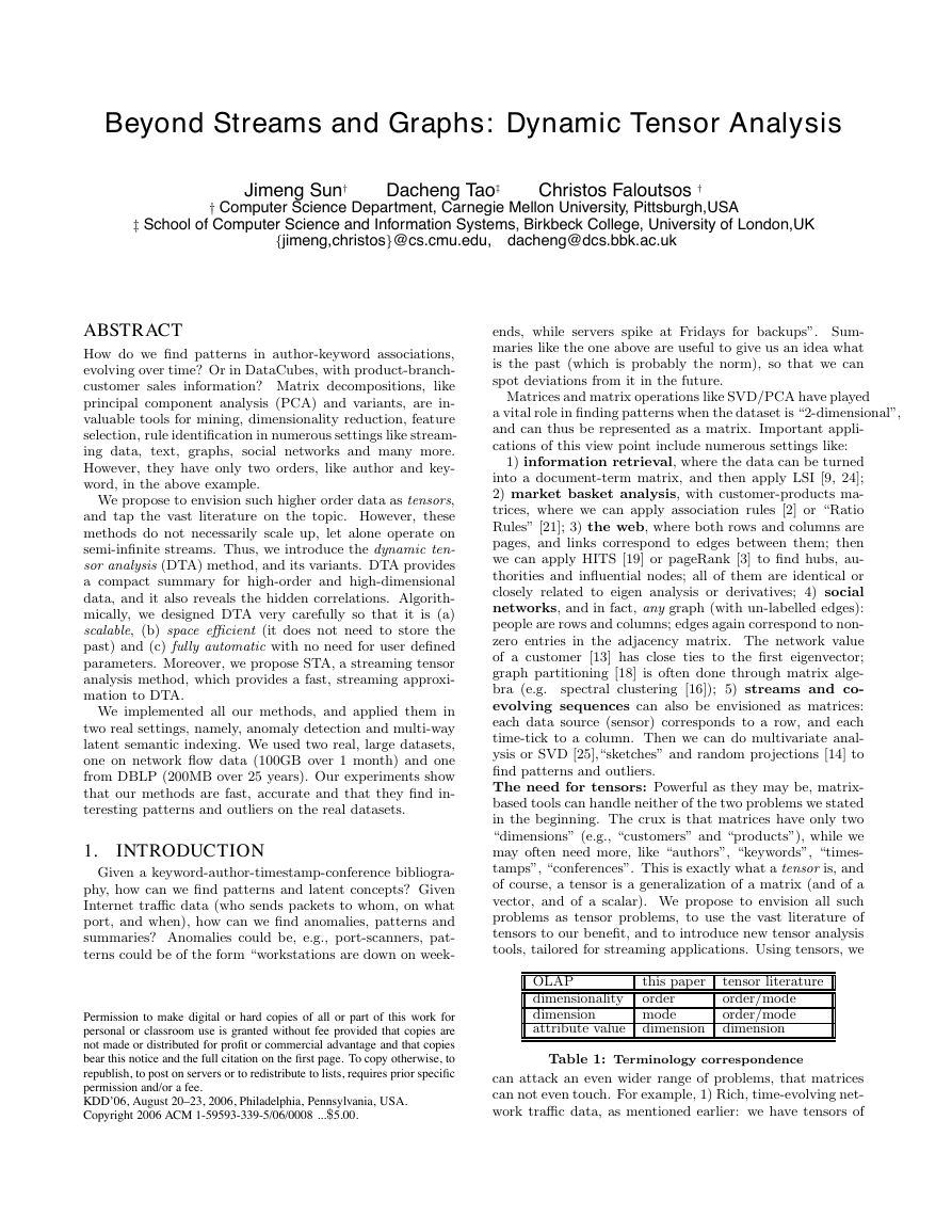BACKGROUND Figure 1: 3rd order tensor of network ﬂow data Therefore, from the data model aspect, we propose to use a more general and expressive model tensor sequences. For the network ﬂow example, the 3rd order tensor for a given time period has three modes: source, destination and port, which can be viewed as a 3D data cube (see Figure 1(a)). An entry (i, j, k) in that tensor (like the small blue cube in Figure 1(a)) has the number of packets from the correspond- ing source (i) to the destination j through port k, during the given time period. The dynamic aspect comes from the fact that new tensors are arriving continuously over time. From the algorithmic aspect, we propose the dynamic and the streaming tensor analysis (DTA and STA) to sum- marize the original tensors into smaller “core” tensors and the “projection matrices” (one for each mode), as shown in Figure 1(b). The projection matrices can be updated incre- mentally over time when a new tensor arrives, and contain valuable information about which, eg., source IP addresses are correlated with which destination IP addresses and des- tination ports, over time. Finally, from the application aspect, we illustrate the anomaly detection and multi-way LSI through DTA/STA. For the former, our method found suspicious Internet activ- ity in a real trace, and it also found the vast majority of injected anomalies (see Section 6). For the latter, we found natural groups of authors, keywords and time intervals, in the DBLP bibliography subset. Our contributions: • The introduction of tensors to streaming analysis. • Two new fast, incremental tools, the dynamic and the streaming tensor analysis (DTA and STA). Here we brieﬂy give the main concepts and terms from principal component analysis (PCA), and from tensor alge- bra, also known as multilinear analysis. 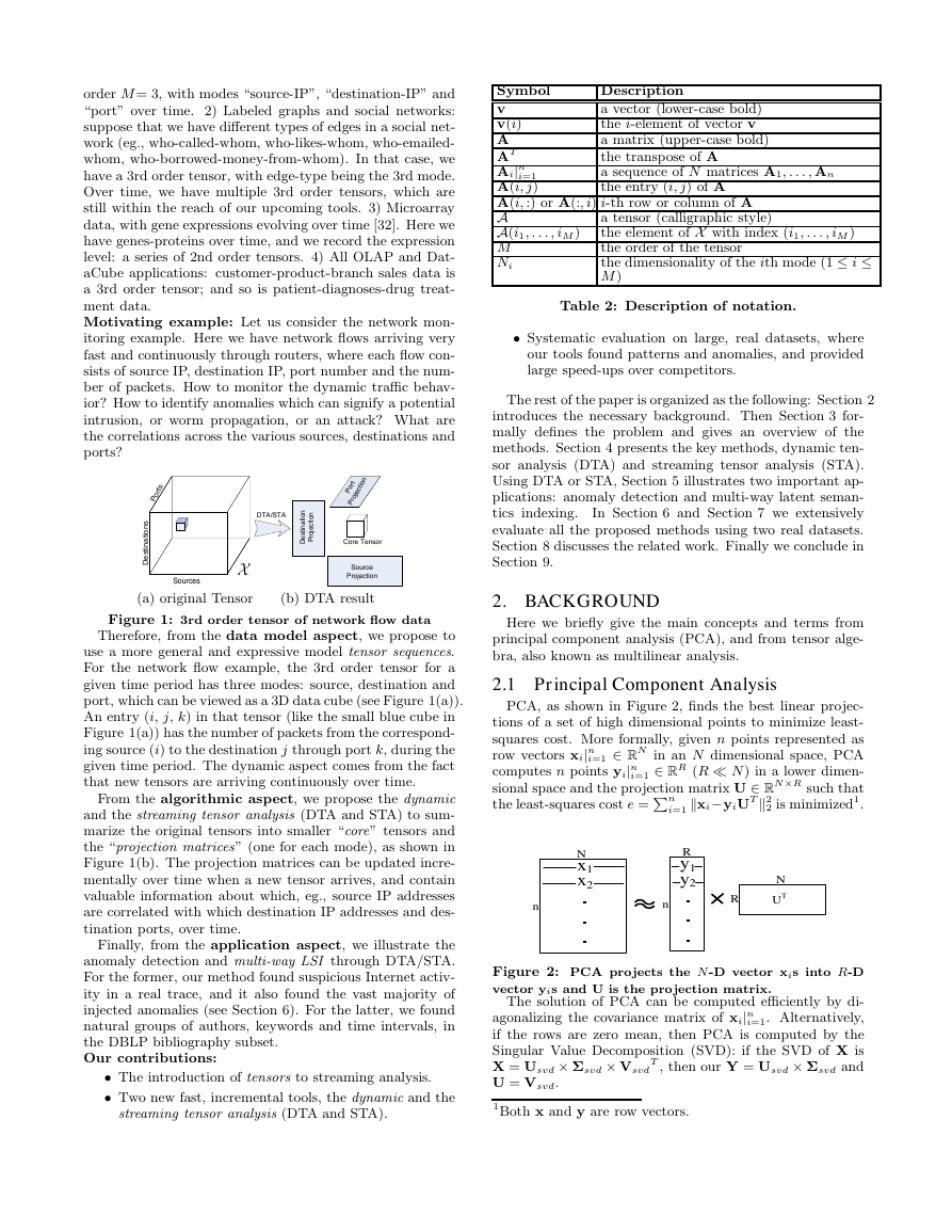2.1 Principal Component Analysis PCA, as shown in Figure 2, ﬁnds the best linear projec- tions of a set of high dimensional points to minimize least- squares cost. More formally, given n points represented as row vectors xi|n i=1 ∈ RN in an N dimensional space, PCA i=1 ∈ RR (R ≪ N ) in a lower dimen- computes n points yi|n sional space and the projection matrix U ∈ RN ×R such that the least-squares cost e = Pn 2 is minimized1. i=1 kxi −yiUT k2 N x1 x2 R y1 y2 N UT R n n Figure 2: PCA projects the N -D vector xis into R-D vector yis and U is the projection matrix. The solution of PCA can be computed eﬃciently by di- agonalizing the covariance matrix of xi|n i=1. Alternatively, if the rows are zero mean, then PCA is computed by the Singular Value Decomposition (SVD): if the SVD of X is T , then our Y = Usvd × Σsvd and X = Usvd × Σsvd × Vsvd U = Vsvd. 1Both x and y are row vectors.

The intuition behind PCA is the following: if X is the author-keyword matrix of the DBLP dataset, then matrix Y is roughly the author-topic, and matrix U is the keyword- topic matrix. 2.2 Multilinear Analysis As mentioned, a tensor of order M closely resembles a Data Cube with M dimensions. Formally, we write an M th order tensor X ∈ RN1×···×NM as X[N1,...,NM ], where Ni (1 ≤ i ≤ M ) is the dimensionality of the ith mode (“di- mension” in OLAP terminology). For brevity, we often omit the subscript [N1, . . . , NM ]. We will also follow the typical conventions, and denote matrices with upper case bold letters (e.g., U) row vectors with lower-case bold letters (e.g., x, scalars with lower-case normal font (e.g., n), and tensors with calligraphic font (e.g., X ). From the tensor literature we need the following deﬁni- tions: Definition 1 (Matricizing or Matrix Unfolding). The mode-d matricizing or matrix unfolding of an M th or- der tensor X ∈ RN1×···×NM are vectors in RNd obtained by keeping index d ﬁxed and varying the other indices. There- fore, the mode-d matricizing X(d) is in R(Qi6=d Ni)×Nd . The mode-d matricizing X is denoted as unfold(X ,d)= X(d). Similarly, the inverse operation is denoted as fold(X(d)). 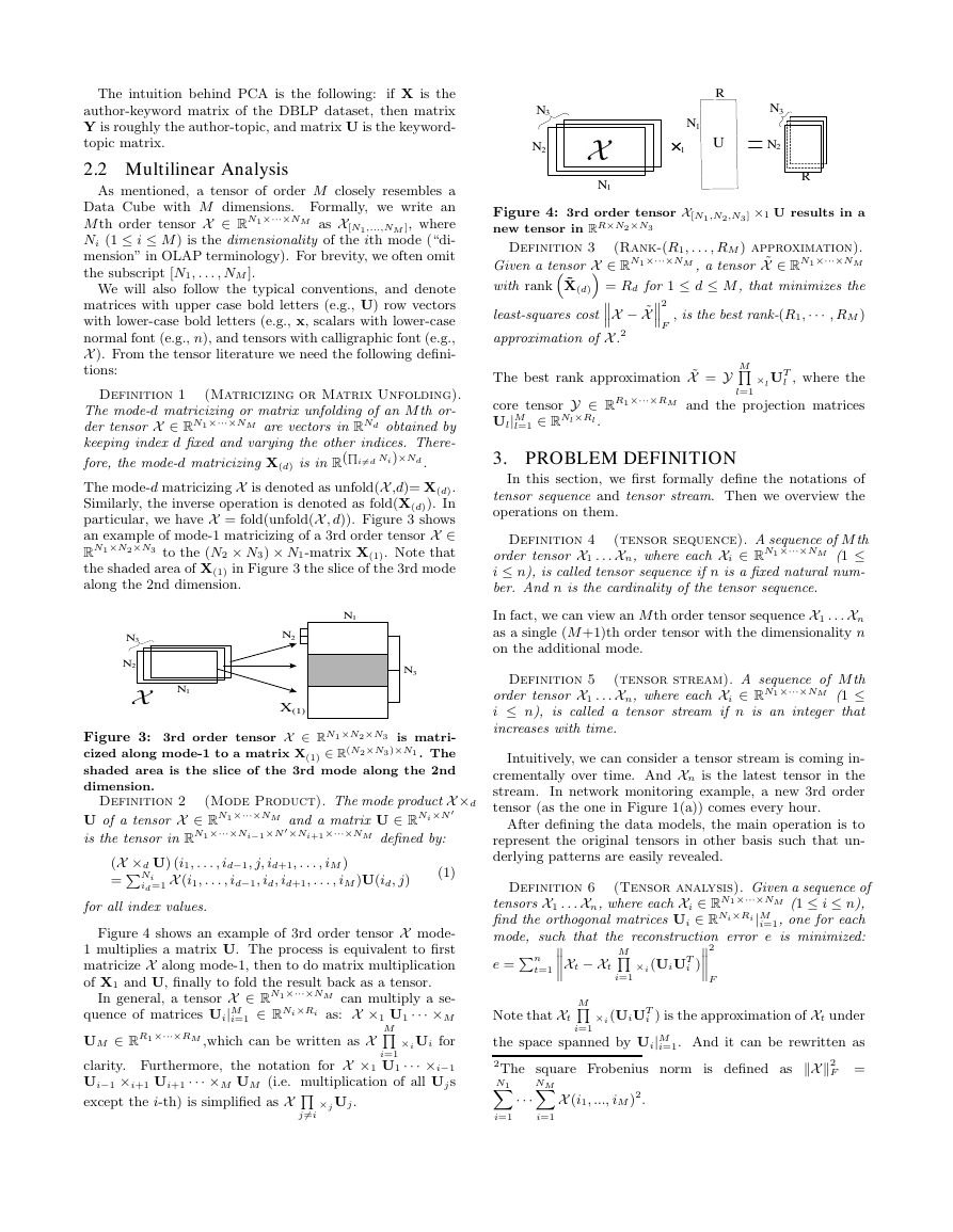In particular, we have X = fold(unfold(X , d)). Figure 3 shows an example of mode-1 matricizing of a 3rd order tensor X ∈ RN1×N2×N3 to the (N2 × N3) × N1-matrix X(1). Note that the shaded area of X(1) in Figure 3 the slice of the 3rd mode along the 2nd dimension. N3 N2 N1 N1 N3 N2 X(1) Figure 3: 3rd order tensor X ∈ RN1×N2×N3 is matri- cized along mode-1 to a matrix X(1) ∈ R(N2×N3)×N1 . The shaded area is the slice of the 3rd mode along the 2nd dimension. Definition 2 (Mode Product). The mode product X ×d U of a tensor X ∈ RN1×···×NM and a matrix U ∈ RNi ×N ′ is the tensor in RN1×···×Ni−1×N ′×Ni+1×···×NM deﬁned by: (X ×d U) (i1, . . . , id−1, j, id+1, . . . , iM ) = PNi id=1 X (i1, . . . , id−1, id, id+1, . . . , iM )U(id, j) (1) for all index values. 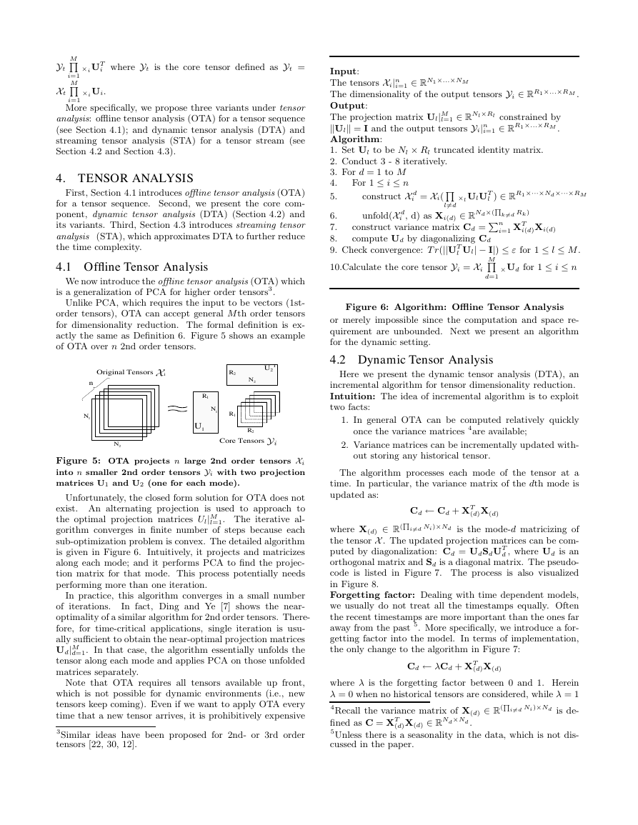Figure 4 shows an example of 3rd order tensor X mode- 1 multiplies a matrix U. The process is equivalent to ﬁrst matricize X along mode-1, then to do matrix multiplication of X1 and U, ﬁnally to fold the result back as a tensor. In general, a tensor X ∈ RN1×···×NM can multiply a se- i=1 ∈ RNi×Ri as: X ×1 U1 · · · ×M quence of matrices Ui|M UM ∈ RR1×···×RM ,which can be written as X M Qi=1 ×i Ui for clarity. Furthermore, the notation for X ×1 U1 · · · ×i−1 Ui−1 ×i+1 Ui+1 · · · ×M UM (i.e. multiplication of all Uj s except the i-th) is simpliﬁed as X Qj6=i ×j Uj. N3 N2 N1 R U N1 1 N3 N2 R Figure 4: 3rd order tensor X[N1 ,N2,N3] ×1 U results in a new tensor in RR×N2×N3 Definition 3 (Rank-(R1, . . . , RM ) approximation). Given a tensor X ∈ RN1×···×NM , a tensor ˜X ∈ RN1×···×NM with rank“ ˜X(d)” = Rd for 1 ≤ d ≤ M , that minimizes the least-squares cost ‚‚‚ , is the best rank-(R1, · · · , RM ) X − ˜X‚‚‚ approximation of X .2 F 2 The best rank approximation ˜X = Y M Ql=1 ×l UT l , where the core tensor Y ∈ RR1×···×RM and the projection matrices Ul|M l=1 ∈ RNl×Rl . 3. PROBLEM DEFINITION In this section, we ﬁrst formally deﬁne the notations of tensor sequence and tensor stream. Then we overview the operations on them. Definition 4 (tensor sequence). A sequence of M th order tensor X1 . . . Xn, where each Xi ∈ RN1×···×NM (1 ≤ i ≤ n), is called tensor sequence if n is a ﬁxed natural num- ber. And n is the cardinality of the tensor sequence. In fact, we can view an M th order tensor sequence X1 . . . Xn as a single (M +1)th order tensor with the dimensionality n on the additional mode. Definition 5 (tensor stream). A sequence of M th order tensor X1 . . . Xn, where each Xi ∈ RN1×···×NM (1 ≤ i ≤ n), is called a tensor stream if n is an integer that increases with time. Intuitively, we can consider a tensor stream is coming in- crementally over time. And Xn is the latest tensor in the stream. In network monitoring example, a new 3rd order tensor (as the one in Figure 1(a)) comes every hour. After deﬁning the data models, the main operation is to represent the original tensors in other basis such that un- derlying patterns are easily revealed. Definition 6 (Tensor analysis). Given a sequence of tensors X1 . . . Xn, where each Xi ∈ RN1×···×NM (1 ≤ i ≤ n), ﬁnd the orthogonal matrices Ui ∈ RNi×Ri |M i=1, one for each mode, such that the reconstruction error e is minimized: t=1 ‚‚‚‚ e = Pn i )‚‚‚‚ ×i (UiUT Xt − Xt F 2 M Qi=1 Note that Xt M Qi=1 ×i (UiUT i ) is the approximation of Xt under the space spanned by Ui|M 2The square Frobenius norm is deﬁned as kX k2 N1 i=1. And it can be rewritten as F = NM X i=1 · · · X i=1 X (i1, ..., iM )2.

M M ×i UT Yt Xt ×i Ui. i where Yt is the core tensor deﬁned as Yt = Qi=1 Qi=1 More speciﬁcally, we propose three variants under tensor analysis: oﬄine tensor analysis (OTA) for a tensor sequence (see Section 4.1); and dynamic tensor analysis (DTA) and streaming tensor analysis (STA) for a tensor stream (see Section 4.2 and Section 4.3). 4. TENSOR ANALYSIS First, Section 4.1 introduces oﬄine tensor analysis (OTA) for a tensor sequence. Second, we present the core com- ponent, dynamic tensor analysis (DTA) (Section 4.2) and its variants. Third, Section 4.3 introduces streaming tensor analysis (STA), which approximates DTA to further reduce the time complexity. 4.1 Ofﬂine Tensor Analysis We now introduce the oﬄine tensor analysis (OTA) which is a generalization of PCA for higher order tensors3. Unlike PCA, which requires the input to be vectors (1st- order tensors), OTA can accept general M th order tensors for dimensionality reduction. The formal deﬁnition is ex- actly the same as Deﬁnition 6. Figure 5 shows an example of OTA over n 2nd order tensors. Original Tensors i n 1N 2N T U2 R2 2N R1 1U 1N R1 R2 Core Tensors Figure 5: OTA projects n large 2nd order tensors Xi into n smaller 2nd order tensors Yi with two projection matrices U1 and U2 (one for each mode). Unfortunately, the closed form solution for OTA does not exist. An alternating projection is used to approach to the optimal projection matrices Ul|M l=1. The iterative al- gorithm converges in ﬁnite number of steps because each sub-optimization problem is convex. The detailed algorithm is given in Figure 6. Intuitively, it projects and matricizes along each mode; and it performs PCA to ﬁnd the projec- tion matrix for that mode. This process potentially needs performing more than one iteration. In practice, this algorithm converges in a small number In fact, Ding and Ye [7] shows the near- of iterations. optimality of a similar algorithm for 2nd order tensors. There- fore, for time-critical applications, single iteration is usu- ally suﬃcient to obtain the near-optimal projection matrices Ud|M d=1. In that case, the algorithm essentially unfolds the tensor along each mode and applies PCA on those unfolded matrices separately. Note that OTA requires all tensors available up front, which is not possible for dynamic environments (i.e., new tensors keep coming). Even if we want to apply OTA every time that a new tensor arrives, it is prohibitively expensive 3Similar ideas have been proposed for 2nd- or 3rd order tensors [22, 30, 12]. i=1 ∈ RN1×...×NM Input: The tensors Xi|n The dimensionality of the output tensors Yi ∈ RR1×...×RM . Output: The projection matrix Ul|M kUlk = I and the output tensors Yi|n Algorithm: 1. Set Ul to be Nl × Rl truncated identity matrix. 2. Conduct 3 - 8 iteratively. 3. For d = 1 to M 4. For 1 ≤ i ≤ n 5. l=1 ∈ RNl×Rl constrained by i=1 ∈ RR1×...×RM . construct X d ×l UlUT l ) ∈ RR1×···×Nd×···×RM i = Xi(Ql6=d unfold(X d 6. 7. 8. 9. Check convergence: T r(||UT construct variance matrix Cd = Pn compute Ud by diagonalizing Cd i , d) as Xi(d) ∈ RNd×(Qk6=d Rk) i=1 XT i(d)Xi(d) l Ul| − I|) ≤ ε for 1 ≤ l ≤ M . 10.Calculate the core tensor Yi = Xi M Qd=1 ×Ud for 1 ≤ i ≤ n Figure 6: Algorithm: Oﬄine Tensor Analysis or merely impossible since the computation and space re- quirement are unbounded. Next we present an algorithm for the dynamic setting. 4.2 Dynamic Tensor Analysis Here we present the dynamic tensor analysis (DTA), an incremental algorithm for tensor dimensionality reduction. Intuition: The idea of incremental algorithm is to exploit two facts: 1. In general OTA can be computed relatively quickly once the variance matrices 4are available; 2. Variance matrices can be incrementally updated with- out storing any historical tensor. The algorithm processes each mode of the tensor at a time. In particular, the variance matrix of the dth mode is updated as: Cd ← Cd + XT (d)X(d) where X(d) ∈ R(Qi6=d Ni)×Nd is the mode-d matricizing of the tensor X . The updated projection matrices can be com- puted by diagonalization: Cd = UdSdUT d , where Ud is an orthogonal matrix and Sd is a diagonal matrix. 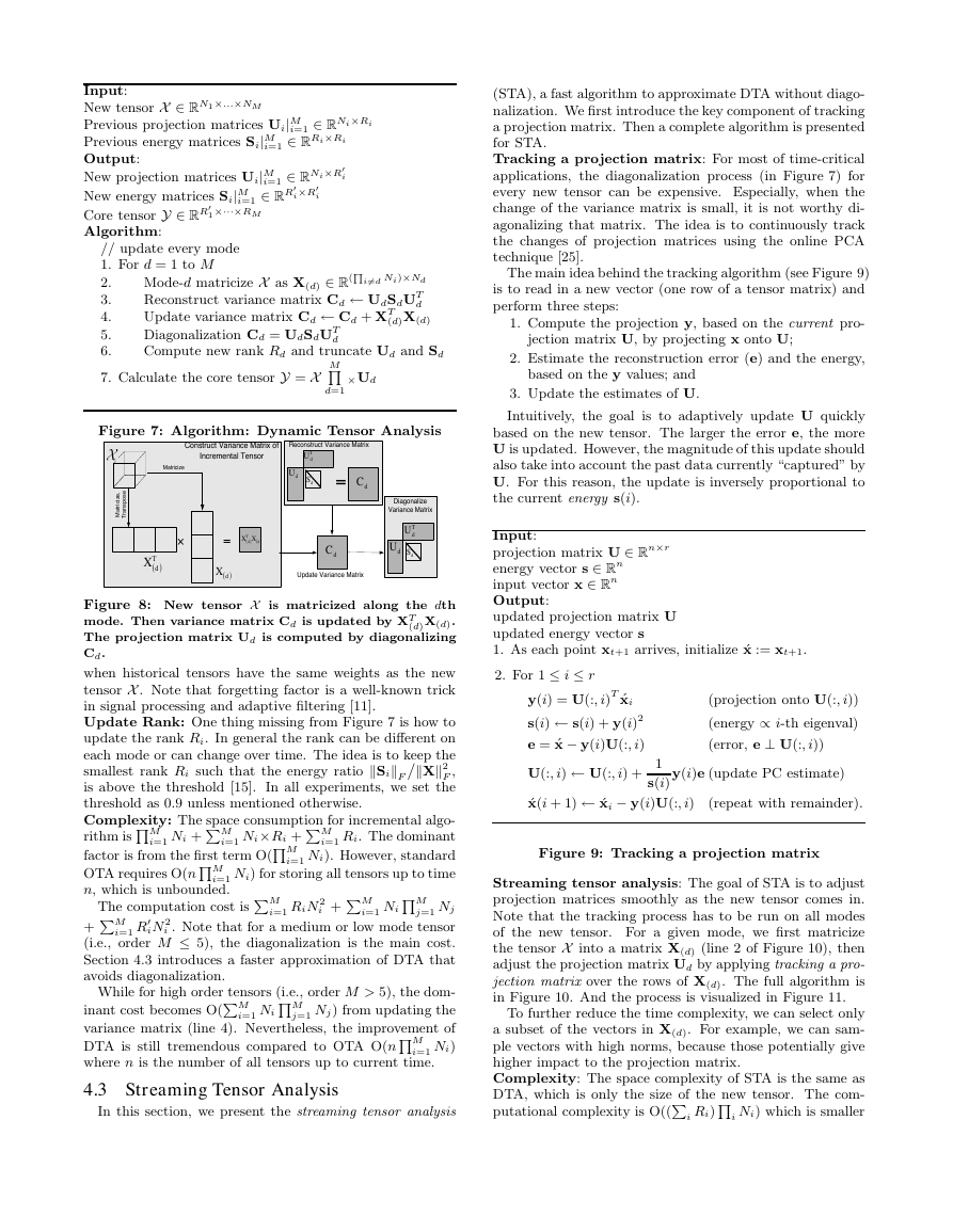The pseudo- code is listed in Figure 7. The process is also visualized in Figure 8. Forgetting factor: Dealing with time dependent models, we usually do not treat all the timestamps equally. Often the recent timestamps are more important than the ones far away from the past 5. More speciﬁcally, we introduce a for- getting factor into the model. In terms of implementation, the only change to the algorithm in Figure 7: Cd ← λCd + XT (d)X(d) where λ is the forgetting factor between 0 and 1. Herein λ = 0 when no historical tensors are considered, while λ = 1 4Recall the variance matrix of X(d) ∈ R(Qi6=d Ni)×Nd is de- ﬁned as C = XT 5Unless there is a seasonality in the data, which is not dis- cussed in the paper. (d)X(d) ∈ RNd×Nd .

Input: New tensor X ∈ RN1×...×NM Previous projection matrices Ui|M Previous energy matrices Si|M Output: New projection matrices Ui|M New energy matrices Si|M Core tensor Y ∈ RR′ Algorithm: i=1 ∈ RR′ 1×···×RM i=1 ∈ RNi×R′ i i×R′ i i=1 ∈ RNi ×Ri i=1 ∈ RRi×Ri // update every mode 1. For d = 1 to M 2. 3. 4. 5. 6. Mode-d matricize X as X(d) ∈ R(Qi6=d Ni)×Nd Reconstruct variance matrix Cd ← UdSdUT d Update variance matrix Cd ← Cd + XT (d)X(d) Diagonalization Cd = UdSdUT d Compute new rank Rd and truncate Ud and Sd 7. Calculate the core tensor Y = X M Qd=1 ×Ud Figure 7: Algorithm: Dynamic Tensor Analysis , i e z c i r t a M Construct Variance Matrix of Incremental Tensor Matricize Reconstruct Variance Matrix T dU dS dU = dC e s o p s n a r T )T dX ( = )dX ( X X T ( d ) Diagonalize Variance Matrix T dU dS dU ( d ) dC Update Variance Matrix Figure 8: New tensor X is matricized along the dth mode. Then variance matrix Cd is updated by XT (d)X(d). The projection matrix Ud is computed by diagonalizing Cd. when historical tensors have the same weights as the new tensor X . Note that forgetting factor is a well-known trick in signal processing and adaptive ﬁltering [11]. Update Rank: One thing missing from Figure 7 is how to update the rank Ri. In general the rank can be diﬀerent on each mode or can change over time. The idea is to keep the smallest rank Ri such that the energy ratio kSikF‹kXk2 F , is above the threshold [15]. In all experiments, we set the threshold as 0.9 unless mentioned otherwise. Complexity: The space consumption for incremental algo- rithm is QM i=1 Ni + PM i=1 Ni ×Ri + PM i=1 Ri. The dominant factor is from the ﬁrst term O(QM i=1 Ni). However, standard OTA requires O(nQM i=1 Ni) for storing all tensors up to time n, which is unbounded. iN 2 i=1 R′ i=1 RiN 2 The computation cost is PM j=1 Nj + PM i . Note that for a medium or low mode tensor (i.e., order M ≤ 5), the diagonalization is the main cost. Section 4.3 introduces a faster approximation of DTA that avoids diagonalization. i=1 Ni QM i + PM i=1 Ni QM While for high order tensors (i.e., order M > 5), the dom- inant cost becomes O(PM j=1 Nj ) from updating the variance matrix (line 4). Nevertheless, the improvement of DTA is still tremendous compared to OTA O(nQM i=1 Ni) where n is the number of all tensors up to current time. 4.3 Streaming Tensor Analysis In this section, we present the streaming tensor analysis (STA), a fast algorithm to approximate DTA without diago- nalization. We ﬁrst introduce the key component of tracking a projection matrix. Then a complete algorithm is presented for STA. Tracking a projection matrix: For most of time-critical applications, the diagonalization process (in Figure 7) for every new tensor can be expensive. Especially, when the change of the variance matrix is small, it is not worthy di- agonalizing that matrix. The idea is to continuously track the changes of projection matrices using the online PCA technique [25]. The main idea behind the tracking algorithm (see Figure 9) is to read in a new vector (one row of a tensor matrix) and perform three steps: 1. Compute the projection y, based on the current pro- jection matrix U, by projecting x onto U; 2. Estimate the reconstruction error (e) and the energy, based on the y values; and 3. Update the estimates of U. Intuitively, the goal is to adaptively update U quickly based on the new tensor. The larger the error e, the more U is updated. However, the magnitude of this update should also take into account the past data currently “captured” by U. For this reason, the update is inversely proportional to the current energy s(i). Input: projection matrix U ∈ Rn×r energy vector s ∈ Rn input vector x ∈ Rn Output: updated projection matrix U updated energy vector s 1. As each point xt+1 arrives, initialize ´x := xt+1. 2. For 1 ≤ i ≤ r y(i) = U(:, i)T ´xi s(i) ← s(i) + y(i)2 e = ´x − y(i)U(:, i) U(:, i) ← U(:, i) + 1 s(i) (projection onto U(:, i)) (energy ∝ i-th eigenval) (error, e ⊥ U(:, i)) y(i)e (update PC estimate) ´x(i + 1) ← ´xi − y(i)U(:, i) (repeat with remainder). Figure 9: Tracking a projection matrix Streaming tensor analysis: The goal of STA is to adjust projection matrices smoothly as the new tensor comes in. Note that the tracking process has to be run on all modes of the new tensor. For a given mode, we ﬁrst matricize the tensor X into a matrix X(d) (line 2 of Figure 10), then adjust the projection matrix Ud by applying tracking a pro- jection matrix over the rows of X(d). The full algorithm is in Figure 10. And the process is visualized in Figure 11. To further reduce the time complexity, we can select only a subset of the vectors in X(d). For example, we can sam- ple vectors with high norms, because those potentially give higher impact to the projection matrix. Complexity: The space complexity of STA is the same as DTA, which is only the size of the new tensor. The com- putational complexity is O((Pi Ri)Qi Ni) which is smaller ·

than DTA (when Ri ≪ Ni). The STA can be further im- proved with random sampling technique, i.e., use only subset of rows of X(d) for update. i=1 ∈ RNi ×Ri i=1 ∈ RRi×Ri Input: New tensor X ∈ RN1×...×NM Old projection matrices Ui|M Old energy matrices Si|M Output: New projection matrices Ui|M New energy matrices Si|M Core tensor Y ∈ RR1×···×RM Algorithm: i=1 ∈ RNi×Ri i=1 ∈ RRi×Ri 1. For d = 1 to M // update every mode 2. 3. 4. Matricize new tensor X as X(d) ∈ R(Qi6=d Ni)×Nd For each column vector x in XT Track a projection matrix (Ud, diag(Si), x) (d) 5. Calculate the core tensor Y = X M Qd=1 ×Ud Figure 10: Algorithm: Streaming Tensor Analysis )T dX ( Matricizing x P o p o u t is Pop out Update iu Update dS dU dS dU Pop out Figure 11: New tensor X is matricized along the dth mode. For every row of Xd, we update the projection matrix Ud. And Sd helps determine the update size. 5. APPLICATIONS After presenting the core technique of tensor analysis, we now illustrate two practical applications of DTA or STA: 1) Anomaly detection, which tries to identify abnormal be- havior across diﬀerent tensors as well as within a tensor; 2) Multi-way latent semantic indexing (LSI), which ﬁnds the correlated dimensions in the same mode and across diﬀer- ent modes. 5.1 Anomaly Detection We envision the abnormal detection as a multi-level screen- ing process, where we try to ﬁnd the anomaly from the broadest level and gradually narrow down to the speciﬁcs. In particular, it can be considered as a three-level process for tensor stream: 1) given a sequence of tensors, identify the abnormal ones; 2) on those suspicious tensors, we locate the abnormal modes; 3) and then ﬁnd the abnormal dimensions of the given mode. In the network monitoring example, the system ﬁrst tries to determine when the anomaly occurs; then it tries to ﬁnd why it occurs by looking at the traﬃc patterns from sources, destinations and ports, respectively; ﬁnally, it narrows down the problem on speciﬁc hosts or ports. For level one (tensor level), we model the abnormality of a tensor X by its reconstruction error: ei = kXi − Yi M Y l=1 ×l UT l kF = kXi − Xi M Y l=1 ×l UlUT l k2 F . For level two (mode level), the reconstruction error of the lth mode only involves one projection matrix Ul for a given tensor X : ed = kX − X ×l UlUT l k2 F . For level three (dimension level), the error of dimension d on the lth mode is just the reconstruction of the tensor slice of dimension d along the lth mode. How much error is too much? We answer this question in the typical way: If the error at time T is enough (say, 2) standard deviations away from the mean error so far, we declare the tensor XT as abnormal. Formally, the condition is as follows: eT +1 ≥ mean“ei|T +1 i=1 ” + α · std“ei|T +1 i=1 ” . 5.2 Multi-way Latent Semantic Indexing The goal of the multi-way LSI is to ﬁnd high correlated di- mensions within the same mode and across diﬀerent modes, and monitor them over time. 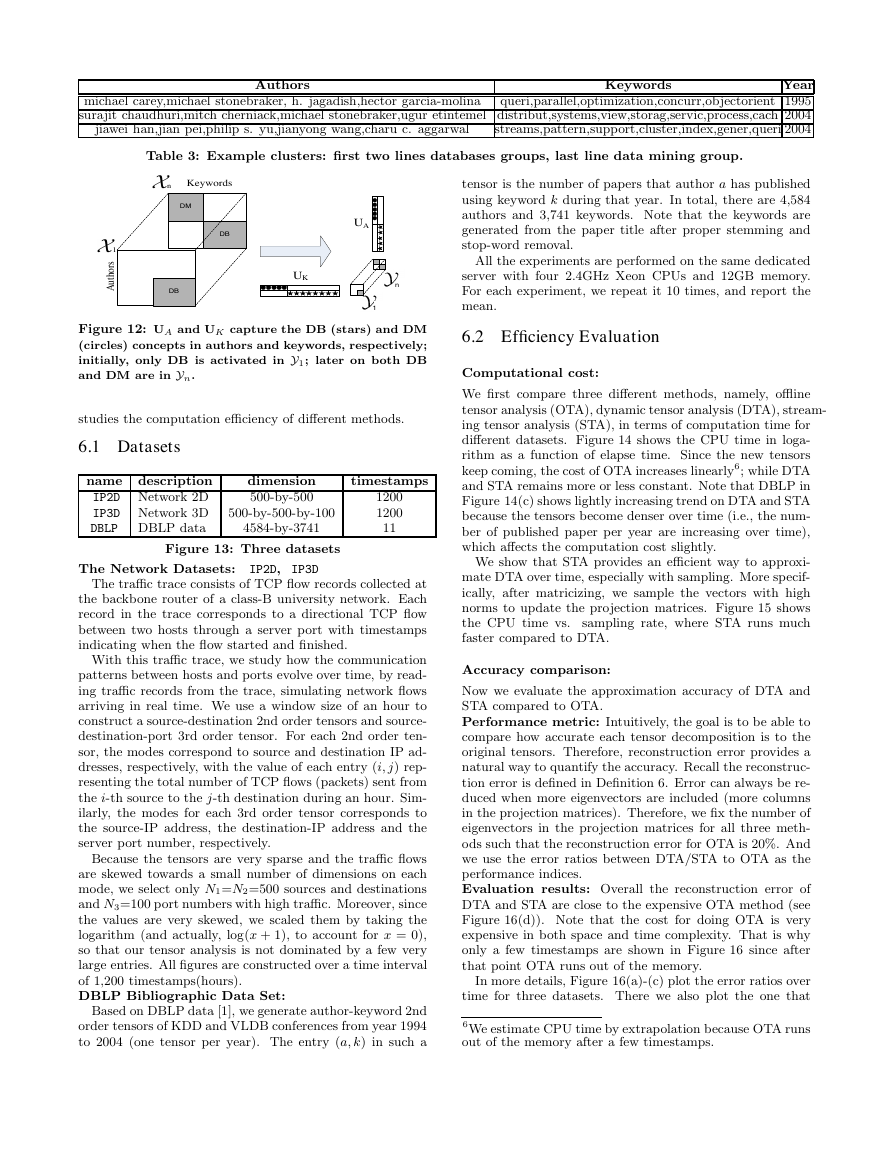Consider the DBLP example, author-keyword over time, Figure 12 shows that initially (in X1) there is only one group, DB, in which all authors and keywords are related to databases; later on (in Xn) two groups appear, namely, databases (DB) and data mining (DM). Correlation within a mode: A projection matrix gives the correlation information among dimensions for a given mode. More speciﬁcally, the dimensions of the lth mode can be grouped based on their values in the columns of Ul. The entries with high absolute values in a column of Ul cor- respond to the important dimensions in the same “concept”. In the DBLP example shown in Figure 12, UK corre- sponds to the keyword concepts. First and second columns are the DB and DM concepts, respectively. The circles of UA and UK indicate the inﬂuential authors and keywords in DM concept, respectively. Similarly, the stars are for DB concept. An example of actual keywords and authors is in Table 3. Correlations across modes: The interesting aspect of DTA is that the core tensor Y provides indications on the correlations of diﬀerent dimensions across diﬀerent modes. More speciﬁcally, a large entry in Y means a high correla- tion between the corresponding columns in all modes. For example in Figure 12, the large values of Yi (in the shaded region) activate the corresponding concepts of the tensor Xi. For simplicity, we described a non-overlapping example, however, groups may overlap which actually happens often in real datasets. Correlations across time: And the core tensor Yis also capture the temporal evolution of concepts. In particular, Y1 only activates the DB concept; while Yn activates both DB and DM concepts. Note that DTA monitors the projection matrices over In this case, the concept space captured by projec- time. tion matrix Uis are also changing over time. 6. EXPERIMENTS In this Section, we evaluate the proposed methods on real datasets. Section 6.1 introduces the datasets. Section 6.2

Year michael carey,michael stonebraker, h. jagadish,hector garcia-molina queri,parallel,optimization,concurr,objectorient 1995 surajit chaudhuri,mitch cherniack,michael stonebraker,ugur etintemel distribut,systems,view,storag,servic,process,cach 2004 streams,pattern,support,cluster,index,gener,queri 2004 jiawei han,jian pei,philip s. yu,jianyong wang,charu c. aggarwal Keywords Authors Table 3: Example clusters: ﬁrst two lines databases groups, last line data mining group. n Keywords DM DB 1 s r o h t u A DB UA n 1 UK tensor is the number of papers that author a has published using keyword k during that year. In total, there are 4,584 authors and 3,741 keywords. Note that the keywords are generated from the paper title after proper stemming and stop-word removal. All the experiments are performed on the same dedicated server with four 2.4GHz Xeon CPUs and 12GB memory. For each experiment, we repeat it 10 times, and report the mean. Figure 12: UA and UK capture the DB (stars) and DM (circles) concepts in authors and keywords, respectively; initially, only DB is activated in Y1; later on both DB and DM are in Yn. 6.2 Efﬁciency Evaluation Computational cost: studies the computation eﬃciency of diﬀerent methods. 6.1 Datasets name description IP2D Network 2D IP3D Network 3D 500-by-500-by-100 DBLP DBLP data dimension 500-by-500 4584-by-3741 timestamps 1200 1200 11 Figure 13: Three datasets The Network Datasets: IP2D, IP3D The traﬃc trace consists of TCP ﬂow records collected at the backbone router of a class-B university network. Each record in the trace corresponds to a directional TCP ﬂow between two hosts through a server port with timestamps indicating when the ﬂow started and ﬁnished. With this traﬃc trace, we study how the communication patterns between hosts and ports evolve over time, by read- ing traﬃc records from the trace, simulating network ﬂows arriving in real time. We use a window size of an hour to construct a source-destination 2nd order tensors and source- destination-port 3rd order tensor. For each 2nd order ten- sor, the modes correspond to source and destination IP ad- dresses, respectively, with the value of each entry (i, j) rep- resenting the total number of TCP ﬂows (packets) sent from the i-th source to the j-th destination during an hour. Sim- ilarly, the modes for each 3rd order tensor corresponds to the source-IP address, the destination-IP address and the server port number, respectively. Because the tensors are very sparse and the traﬃc ﬂows are skewed towards a small number of dimensions on each mode, we select only N1=N2=500 sources and destinations and N3=100 port numbers with high traﬃc. Moreover, since the values are very skewed, we scaled them by taking the logarithm (and actually, log(x + 1), to account for x = 0), so that our tensor analysis is not dominated by a few very large entries. All ﬁgures are constructed over a time interval of 1,200 timestamps(hours). DBLP Bibliographic Data Set: Based on DBLP data [1], we generate author-keyword 2nd order tensors of KDD and VLDB conferences from year 1994 to 2004 (one tensor per year). 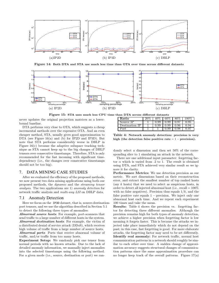The entry (a, k) in such a We ﬁrst compare three diﬀerent methods, namely, oﬄine tensor analysis (OTA), dynamic tensor analysis (DTA), stream- ing tensor analysis (STA), in terms of computation time for diﬀerent datasets. Figure 14 shows the CPU time in loga- rithm as a function of elapse time. Since the new tensors keep coming, the cost of OTA increases linearly6; while DTA and STA remains more or less constant. Note that DBLP in Figure 14(c) shows lightly increasing trend on DTA and STA because the tensors become denser over time (i.e., the num- ber of published paper per year are increasing over time), which aﬀects the computation cost slightly. We show that STA provides an eﬃcient way to approxi- mate DTA over time, especially with sampling. More specif- ically, after matricizing, we sample the vectors with high norms to update the projection matrices. Figure 15 shows the CPU time vs. sampling rate, where STA runs much faster compared to DTA. Accuracy comparison: Now we evaluate the approximation accuracy of DTA and STA compared to OTA. Performance metric: Intuitively, the goal is to be able to compare how accurate each tensor decomposition is to the original tensors. Therefore, reconstruction error provides a natural way to quantify the accuracy. Recall the reconstruc- tion error is deﬁned in Deﬁnition 6. Error can always be re- duced when more eigenvectors are included (more columns in the projection matrices). Therefore, we ﬁx the number of eigenvectors in the projection matrices for all three meth- ods such that the reconstruction error for OTA is 20%. And we use the error ratios between DTA/STA to OTA as the performance indices. Evaluation results: Overall the reconstruction error of DTA and STA are close to the expensive OTA method (see Figure 16(d)). Note that the cost for doing OTA is very expensive in both space and time complexity. That is why only a few timestamps are shown in Figure 16 since after that point OTA runs out of the memory. In more details, Figure 16(a)-(c) plot the error ratios over time for three datasets. There we also plot the one that 6We estimate CPU time by extrapolation because OTA runs out of the memory after a few timestamps.

103 102 101 ) c e s ( e m i t U P C 100 0 OTA DTA STA 20 40 time 60 80 100 102 ) c e s ( e m i t U P C 101 0 OTA DTA STA 102 ) c e s ( e m i t U P C OTA DTA STA 20 40 time 60 80 100 1994 1996 1998 2000 2002 2004 year (a)IP2D (b) IP3D (c) DBLP Figure 14: Both DTA and STA use much less time than OTA over time across diﬀerent datasets 1.6 1.4 1.2 1 0.8 0.6 0.4 ) c e s ( e m i t 0.2 100% DTA STA 12 10 8 6 4 2 ) c e s ( e m i t 75% 50% sampling percentage 25% (a) IP2D 0 100% 45 40 35 30 25 20 15 10 5 ) c e s ( e m i t DTA STA 75% 50% sampling percentage 25% 0 100% 75% 50% sampling percentage (b) IP3D (c) DBLP DTA STA 25% Figure 15: STA uses much less CPU time than DTA across diﬀerent datasets never updates the original projection matrices as a lower- bound baseline. DTA performs very close to OTA, which suggests a cheap incremental methods over the expensive OTA. And an even cheaper method, STA, usually gives good approximation to DTA (see Figure 16(a) and (b) for IP2D and IP3D). But note that STA performs considerably worse in DBLP in Figure 16(c) because the adaptive subspace tracking tech- nique as STA cannot keep up to the big changes of DBLP tensors over consecutive timestamps. Therefore, STA is only recommended for the fast incoming with signiﬁcant time- dependency (i.e., the changes over consecutive timestamps should not be too big). 7. DATA MINING CASE STUDIES After we evaluated the eﬃciency of the proposed methods, we now present two data mining applications using both our proposed methods, the dynamic and the streaming tensor analysis. The two applications are 1) anomaly detection for network traﬃc analysis and multi-way LSI on DBLP data. 7.1 Anomaly Detection Here we focus on the IP3D dataset, that is, source-destination- port tensors, and we use the algorithm described in Section 5.1 to detect the following three types of anomalies: Abnormal source hosts: For example, port-scanners that send traﬃc to a large number of diﬀerent hosts in the system. Abnormal destination hosts: For example, the victim of a distributed denial of service attack (DDoS), which receives high volume of traﬃc from a large number of source hosts. Abnormal ports: Ports that receive abnormal volume of traﬃc, and/or traﬃc from too many hosts. Experiment Setup: We randomly pick one tensor from normal periods with no known attacks. Due to the lack of detailed anomaly information, we manually inject anomalies into the selected timestamps using the following method. For a given mode (i.e., source, destination or port) we ran- Ratio Source IP Destination IP Port 20% 40% 60% 80% 100% 0.95 0.94 0.97 0.99 0.99 0.99 0.97 0.96 0.98 0.99 0.99 1 1 1 1 Table 4: Network anomaly detection: precision is very high (the detection false positive rate = 1 − precision). domly select a dimension and then set 50% of the corre- sponding slice to 1 simulating an attack in the network. There are one additional input parameter: forgetting fac- tor α which is varied from .2 to 1. The result is obtained using DTA, and STA achieved very similar result so we ig- nore it for clarity. Performance Metrics: We use detection precision as our metric. We sort dimensions based on their reconstruction error, and extract the smallest number of top ranked hosts (say k hosts) that we need to select as suspicious hosts, in order to detect all injected abnormal host (i.e., recall = 100% with no false negatives). Precision thus equals 1/k, and the false positive rate equals 1 − precision. We inject only one abnormal host each time. And we repeat each experiment 100 times and take the mean. forgetting fac- Results: Table 4 shows the precision vs. tor for detecting three diﬀerent anomalies. Although the precision remains high for both types of anomaly detection, we achieve a higher precision when forgetting factor is low meaning it forgets faster. This is because the attacks we in- jected take place immediately which do not depend on the past; in this case, fast forgetting is good. For more elaborate attacks, the forgetting factor may need to be set diﬀerently. Identify real anomaly: For network traﬃc, normal host communication patterns in a network should roughly be sim- ilar to each other over time. A sudden change of approxi- mation accuracy suggests structural changes of communica- tion patterns since the same approximation procedure can no longer keep track of the overall patterns. Figure 17(a)

分享到：

赞收藏

资料库

张量子空间算法.pdf

相关推荐

开发技术

热门标签

最新资料