IEEE TRANSACTIONS ON PATTERN ANALYSIS AND MACHINE INTELLIGENCE, VOL. 29, NO. 6,
JUNE 2007
915
Dynamic Texture Recognition Using
Local Binary Patterns with an
Application to Facial Expressions
Guoying Zhao and Matti Pietika¨ inen, Senior Member, IEEE
Abstract—Dynamic texture (DT) is an extension of texture to the temporal domain. Description and recognition of DTs have attracted
growing attention. In this paper, a novel approach for recognizing DTs is proposed and its simplifications and extensions to facial image
analysis are also considered. First, the textures are modeled with volume local binary patterns (VLBP), which are an extension of the
LBP operator widely used in ordinary texture analysis, combining motion and appearance. To make the approach computationally
simple and easy to extend, only the co-occurrences of the local binary patterns on three orthogonal planes (LBP-TOP) are then
considered. A block-based method is also proposed to deal with specific dynamic events such as facial expressions in which local
information and its spatial locations should also be taken into account. In experiments with two DT databases, DynTex and
Massachusetts Institute of Technology (MIT), both the VLBP and LBP-TOP clearly outperformed the earlier approaches. The proposed
block-based method was evaluated with the Cohn-Kanade facial expression database with excellent results. The advantages of our
approach include local processing, robustness to monotonic gray-scale changes, and simple computation.
Index Terms—Temporal texture, motion, facial image analysis, facial expression, local binary pattern.
Ç
1 INTRODUCTION
foliage,
DYNAMIC or temporal textures are textures with motion
[1]. They encompass the class of video sequences that
exhibit some stationary properties in time [2]. There are lots
of dynamic textures (DTs) in the real world, including sea
waves, smoke,
fire, shower, and whirlwind.
Description and recognition of DT are needed, for example,
in video retrieval systems, which have attracted growing
attention. Because of their unknown spatial and temporal
extent, the recognition of DT is a challenging problem
compared with the static case [3]. Polana and Nelson
classified visual motion into activities, motion events, and
DTs [4]. Recently, a brief survey of DT description and
recognition was given by Chetverikov and Pe´teri [5].
Key issues concerning DT recognition include:
1.
combining motion features with appearance features;
2. processing locally to catch the transition information
in space and time, for example, the passage of burning
fire changing gradually from a spark to a large fire;
3. defining features that are robust against
image
transformations such as rotation;
insensitivity to illumination variations;
computational simplicity; and
4.
5.
6. multiresolution analysis. To our knowledge, no
previous method satisfies all of these requirements.
. The authors are with the Machine Vision Group, Department of Electrical
and Information Engineering, University of Oulu, PO Box 4500, FI-90014
Finland. E-mail: {gyzhao, mkp}@ee.oulu.fi.
Manuscript received 1 June 2006; revised 4 Oct. 2006; accepted 16 Jan. 2007;
published online 8 Feb. 2007.
Recommended for acceptance by B.S. Manjunath.
For information on obtaining reprints of this article, please send e-mail to:
tpami@computer.org, and reference IEEECS Log Number TPAMI-0413-0606.
Digital Object Identifier no. 10.1109/TPAMI.2007.1110.
To address these issues, we propose a novel, theoretically
and computationally simple approach based on local binary
patterns. First, the textures are modeled with volume local
binary patterns (VLBP), which are an extension of the local
binary patterns (LBP) operator widely used in ordinary
texture analysis [6], combining the motion and appearance.
The texture features extracted in a small local neighborhood
of the volume are not only insensitive with respect to
translation and rotation, but also robust with respect to
monotonic gray-scale changes caused,
for example, by
illumination variations. To make the VLBP computationally
simple and easy to extend, only the co-occurrences on three
separated planes are then considered. The textures are
modeled with concatenated Local Binary Pattern histo-
grams from Three Orthogonal Planes (LBP-TOP). The
circular neighborhoods are generalized to elliptical sam-
pling to fit the space-time statistics.
As our approach involves only local processing, we are
allowed to take a more general view of DT recognition,
extending it to specific dynamic events such as facial
expressions. A block-based approach combining pixel-level,
region-level, and volume-level features is proposed for
dealing with such nontraditional DTs in which local informa-
tion and its spatial locations should also be taken into account.
This will make our approach a highly valuable tool for many
potential computer vision applications. For example, the
human face plays a significant role in verbal and nonverbal
communication. Fully automatic and real-time facial expres-
sion recognition could find many applications, for instance, in
human-computer interaction, biometrics, telecommunica-
tions, and psychological research. Most of the research on
facial expression recognition has been based on static images
[7], [8], [9], [10], [11], [12], [13]. Some research on using facial
dynamics has also been carried out [14], [15], [16]; however,
reliable segmentation of the lips and other moving facial parts
in natural environments has proven to be a major problem.
0162-8828/07/$25.00 ß 2007 IEEE
Published by the IEEE Computer Society
�
916
IEEE TRANSACTIONS ON PATTERN ANALYSIS AND MACHINE INTELLIGENCE, VOL. 29, NO. 6,
JUNE 2007
Our approach is completely different, avoiding error-prone
segmentation.
2 RELATED WORK
Chetverikov and Pe´teri [5] placed the existing approaches of
temporal texture recognition into five classes: methods
based on optic flow, methods computing geometric proper-
ties in the spatiotemporal domain, methods based on local
spatiotemporal filtering, methods using global spatiotem-
poral transforms and, finally, model-based methods that
use estimated model parameters as features.
The methods based on optic flow [3], [4], [17], [18], [19],
[20], [21], [22], [23], [24] are currently the most popular ones
[5], because optic flow estimation is a computationally
efficient and natural way to characterize the local dynamics
of a temporal texture. Pe´teri and Chetverikov [3] proposed a
method that combines normal flow features with periodicity
features, in an attempt to explicitly characterize motion
magnitude, directionality, and periodicity. Their features
are rotation invariant, and the results are promising.
However, they did not consider the multiscale properties
of DT. Lu et al. proposed a new method using spatiotemporal
multiresolution histograms based on velocity and accelera-
tion fields [21]. Velocity and acceleration fields of different
spatiotemporal resolution image sequences were accurately
estimated by the structure tensor method. This method is
also rotation invariant and provides local directionality
information. Fazekas and Chetverikov compared normal
flow features and regularized complete flow features in DT
classification [25]. They concluded that normal flow contains
information on both dynamics and shape.
Saisan et al. [26] applied a DT model [1] to the recognition
of 50 different temporal textures. Despite this success, their
method assumed stationary DTs that are well segmented in
space and time and the accuracy drops drastically if they are
not. Fujita and Nayar [27] modified the approach [26] by
using impulse responses of state variables to identify model
and texture. Their approach showed less sensitivity to
nonstationarity. However, the problem of heavy computa-
tional load and the issues of scalability and invariance remain
open. Fablet and Bouthemy introduced temporal co-occur-
rence [19], [20] that measures the probability of co-occurrence
in the same image location of two normal velocities (normal
flow magnitudes) separated by certain temporal intervals.
Recently, Smith et al. dealt with video texture indexing using
spatiotemporal wavelets [28]. Spatiotemporal wavelets can
decompose motion into local and global, according to the
desired degree of detail.
Otsuka et al. [29] assumed that DTs can be represented by
moving contours whose motion trajectories can be tracked.
They considered trajectory surfaces within 3D spatiotempor-
al volume data and extracted temporal and spatial features
based on the tangent plane distribution. The spatial features
include the directionality of contour arrangement and the
scattering of contour placement. The temporal features
characterize the uniformity of velocity components, the ash
motion ratio, and the occlusion ratio. These features were
used to classify four DTs. Zhong and Scarlaro [30] modified
[29] and used 3D edges in the spatiotemporal domain. Their
DT features were computed for voxels taking into account the
spatiotemporal gradient.
It appears that nearly all of the research on DT recognition
has considered textures to be more or less “homogeneous,”
that is, the spatial locations of image regions are not taken into
account. The DTs are usually described with global features
computed over the whole image, which greatly limits the
applicability of DT recognition. Using only global features for
face or facial expression recognition, for example, would not
be effective since much of the discriminative information in
facial images is local, such as mouth movements. In their
recent work, Aggarwal et al. [31] adopted the Autoregressive
and Moving Average (ARMA) framework of Doretto et al. [2]
for video-based face recognition, demonstrating that tempor-
al information contained in facial dynamics is useful for face
recognition. In this approach, the use of facial appearance
information is very limited. We are not aware of any DT-
based approaches to facial expression recognition [7], [8], [9].
3 VOLUME LOCAL BINARY PATTERNS (VLBP)
The main difference between DT and ordinary texture is that
the notion of self-similarity, central to conventional image
texture,
is extended to the spatiotemporal domain [5].
Therefore, combining motion and appearance to analyze
DT is well justified. Varying lighting conditions greatly affect
the gray-scale properties of DT. At the same time, the textures
may also be arbitrarily oriented, which suggests using
rotation-invariant features. It is important, therefore, to
define features that are robust with respect to gray-scale
changes, rotations, and translation. In this paper, we propose
the use of VLBP (which could also be called 3D-LBP) to
address these problems [32].
3.1 Basic VLBP
To extend LBP to DT analysis, we define DT V in a local
neighborhood of a monochrome DT sequence as the joint
distribution v of the gray levels of 3P þ 3ðP > 1Þ image
pixels. P is the number of local neighboring points around
the central pixel in one frame:
V ¼ vðgtc�L;c; gtc�L;0;��� ; gtc�L;P�1; gtc;c; gtc;0;
��� ; gtc;P�1; gtcþL;0;��� ; gtcþL;P�1; gtcþL;cÞ;
ð1Þ
where the gray value gtc;c corresponds to the gray value of
the center pixel of the local volume neighborhood, gtc�L;c
and gtcþL;c correspond to the gray value of the center pixel
in the previous and posterior neighboring frames with time
interval L; gt;pðt ¼ tc � L; tc; tc þ L; p ¼ 0;��� ; P � 1Þ corre-
spond to the gray values of P equally spaced pixels on a
circle of radius RðR > 0Þ in image t, which form a circularly
symmetric neighbor set.
the
coordinates of gtc;p are given by ðxc þ R cosð2�p=PÞ; yc �
R sinð2�p=PÞ; tcÞ and the coordinates of gtc�L;p are given by
ðxc þ R cosð2�p=PÞ; yc � R sinð2�p=PÞ; tc � LÞ. The values of
the neighbors that do not fall exactly on pixels are estimated
by bilinear interpolation.
Suppose the coordinates of gtc;c are ðxc; yc; tcÞ,
To get the gray-scale invariance, the distribution is
thresholded similar to that in [6]. The gray value of the
volume center pixelðgtc;cÞ is subtracted from the gray values of
�
ZHAO AND PIETIKA¨ INEN: DYNAMIC TEXTURE RECOGNITION USING LOCAL BINARY PATTERNS WITH AN APPLICATION TO FACIAL...
917
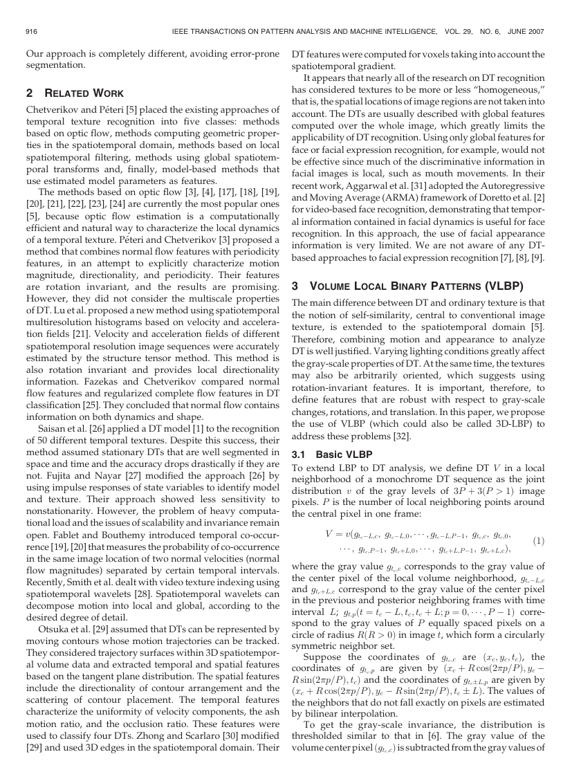
Fig. 1. Procedure of V LBP1;4;1.
the circularly symmetric neighborhood gt;pðt ¼ tc � L; tc;
tc þ L; p ¼ 0;��� ; P � 1Þ, giving
V ¼ vðgtc�L;c � gtc;c; gtc�L;0 � gtc;c;��� ;
gtc�L;P�1 � gtc;c; gtc;c; gtc;0 � gtc;c;��� ;
gtc;P�1 � gtc;c; gtcþL;0 � gtc;c;��� ;
gtcþL;P�1 � gtc;c; gtcþL;c � gtc;cÞ:
ð2Þ
Then, we assume that differences gt;p � gtc;c are indepen-
dent of gtc;c, which allow us to factorize (2):
V � vðgtc;cÞvðgtc�L;c � gtc;c; gtc�L;0 � gtc;c;��� ;
gtc�L;P�1 � gtc;c; gtc;0 � gtc;c;��� ; gtc;P�1 � gtc;c;
gtcþL;0 � gtc;c;��� ; gtcþL;P�1 � gtc;c; gtcþL;c � gtc;cÞ:
In practice, exact independence is not warranted; hence,
the factorized distribution is only an approximation of the
joint distribution. However, we are willing to accept a
possible small loss of information as it allows us to achieve
invariance with respect to shifts in gray scale. Thus, similar to
LBP in ordinary texture analysis [6], the distribution vðgtc;cÞ
describes the overall luminance of the image, which is
unrelated to the local image texture and, consequently, does
not provide useful information for DT analysis. Hence, much
of the information in the original joint gray-level distribution
(1) is conveyed by the joint difference distribution:
V1 ¼ vðgtc�L;c � gtc;c; gtc�L;0 � gtc;c;��� ;
gtc�L;P�1 � gtc;c; gtc;0 � gtc;c;��� ; gtc;P�1 � gtc;c;
gtcþL;0 � gtc;c;��� ; gtcþL;P�1 � gtc;c; gtcþL;c � gtc;cÞ:
This is a highly discriminative texture operator.
It
records the occurrences of various patterns in the neighbor-
in a ð2ðP þ 1Þ þ P ¼ 3P þ 2Þ-dimen-
hood of each pixel
sional histogram.
We achieve invariance with respect to the scaling of the
gray scale by considering simply the signs of the differences
instead of their exact values:
�
V2 ¼ v
sðgtc�L;c � gtc;cÞ; sðgtc�L;0 � gtc;cÞ;��� ;
sðgtc�L;P�1 � gtc;cÞ; sðgtc;0 � gtc;cÞ;��� ;
�
sðgtc;P�1 � gtc;cÞ; sðgtcþL;0 � gtc;cÞ;��� ;
�
sðgtcþL;P�1 � gtc;cÞ; sðgtcþL;c � gtc;cÞ
;
�
ð3Þ
ð4Þ
where sðxÞ ¼ 1; x � 0
0; x < 0
.
To simplify the expression of V2, we use V2 ¼ vðv0;��� ;
vq;��� ; v3Pþ1Þ, and q corresponds to the index of values in
V2 orderly. By assigning a binomial factor 2q for each
sign sðgt;p � gtc;cÞ, we transform (3) into a unique V LBPL;P ;R
number that characterizes the spatial structure of the local
volume DT:
V LBPL;P ;R ¼
X
3Pþ1
vq2q:
q¼0
Fig. 1 shows the whole computing procedure for
V LBP1;4;1. We begin by sampling neighboring points in
the volume and then thresholding every point
in the
neighborhood with the value of the center pixel to get a
binary value. Finally, we produce the VLBP code by
�
918
IEEE TRANSACTIONS ON PATTERN ANALYSIS AND MACHINE INTELLIGENCE, VOL. 29, NO. 6,
JUNE 2007
multiplying the thresholded binary values with weights
given to the corresponding pixel and we sum up the result.
Let us assume we are given an X � Y � T DT ðxc 2
f0;��� ; X � 1g; yc 2 f0;��� ; Y � 1g; tc 2 f0;��� ; T � 1gÞ.
In
calculating V LBPL;P ;R distribution for this DT, the central
part is only considered because a sufficiently large neighbor-
hood cannot be used on the borders in this 3D space. The
basic VLBP code is calculated for each pixel in the cropped
portion of the DT, and the distribution of the codes is used as
a feature vector, denoted by D:
�
�
; x 2 Rd e;��� ; X � 1 � Rd e
g; t 2 Ld e;��� ; T � 1 � Ld e
f
f
g;
g:
D ¼ v V LBPL;P ;Rðx; y; tÞ
y 2 Rd e;��� ; Y � 1 � Rd e
f
The histograms are normalized with respect to volume
size variations by setting the sum of their bins to unity.
Because the DT is viewed as sets of volumes and their
features are extracted on the basis of those volume textons,
VLBP combines the motion and appearance to describe DTs.
3.2 Rotation Invariant VLBP
DT may also be arbitrarily oriented, so they also often rotate in
the videos. The most important difference between rotation in
a still texture image and DT is that the whole sequence of DT
rotates around one axis or multiaxes (if the camera rotates
during capturing), whereas the still texture rotates around
one point. We cannot therefore deal with VLBP as a whole to
get a rotation invariant code, as in [6], which assumed rotation
around the center pixel in the static case. We first divide the
whole VLBP code in (3) into five parts:
�
V2 ¼ v
½sðgtc�L;c � gtc;cÞ;
½sðgtc�L;0 � gtc;cÞ;��� ; sðgtc�L;P�1 � gtc;cÞ;
½sðgtc;0 � gtc;cÞ;��� ; sðgtc;P�1 � gtc;cÞ;
½sðgtcþL;0 � gtc;cÞ;��� ; sðgtcþL;P�1 � gtc;cÞ;
½sðgtcþL;c � gtc;cÞ
�
:
Then, we mark those as VpreC, VpreN , VcurN , VposN , and VposC
in order, and VpreN , VcurN , and VposN represent the LBP code in
the previous, current, and posterior frames, respectively,
whereas VpreC and VposC represent the binary values of the
center pixels in the previous and posterior frames:
X
P�1
p¼0
LBPt;P ;R ¼
sðgt;p � gtc;cÞ2p; t ¼ tc � L; tc; tc þ L:
ð5Þ
Using (5), we can get LBPtc�L;P ;R, LBPtc;P ;R, and
LBPtcþL;P ;R.
To remove the effect of rotation, we use
n
L;P ;R ¼ min
�
V LBPL;P ;R and 23Pþ1
�
V LBP ri
þ ROLðRORðLBPtcþL;P ;R; iÞ; 2P þ 1Þ
þ ROLðRORðLBPtc;P ;R; iÞ; P þ 1Þ
þ ROLðRORðLBPtc�L;P ;R; iÞ; 1Þ
þ ðV LBPL;P ;R and 1Þji ¼ 0; 1;��� ; P � 1
ð6Þ
o
;
where RORðx; iÞ performs a circular bitwise right shift on
the P -bit number x i times [6] and ROLðy; jÞ performs a
bitwise left shift on the 3P þ 2-bit number y j times. In
terms of image pixels, (6) simply corresponds to rotating the
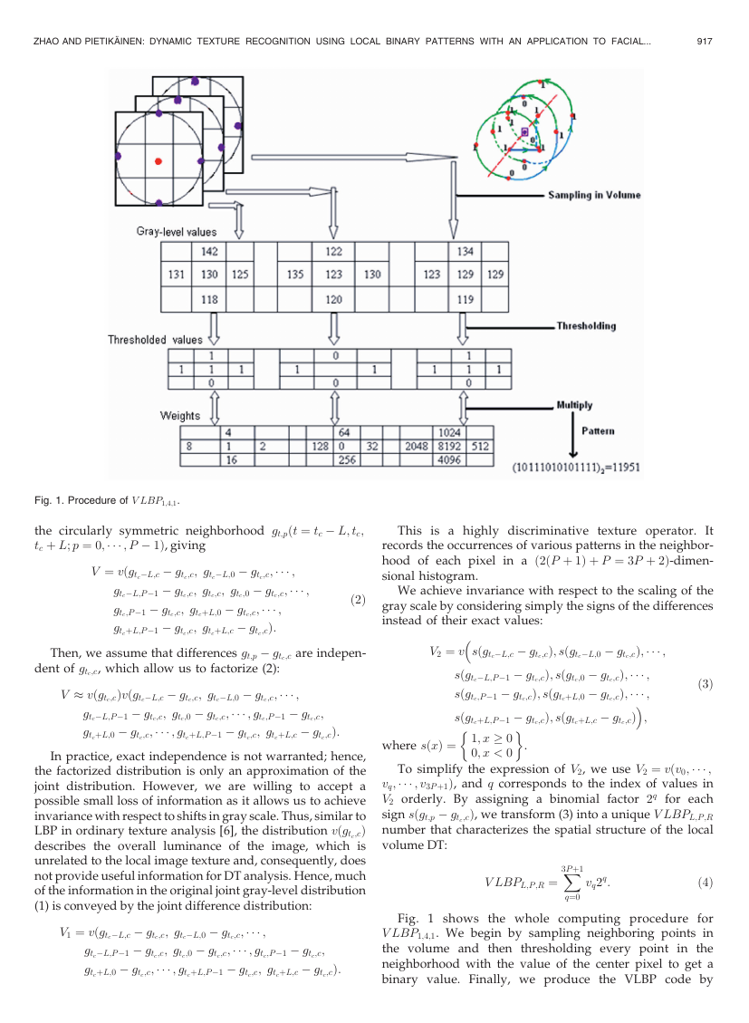
Fig. 2. The number of features versus the number of LBP codes.
neighbor set in three separate frames clockwise and this
happens synchronously so that a minimal value is selected
as the VLBP rotation invariant code.
For example, for the original VLBP code ð1; 1010;
1101; 1100; 1Þ2, its codes after rotating clockwise 90, 180,
and 270 degrees are ð1; 0101; 1110; 0110; 1Þ2, ð1; 1010; 0111;
0011; 1Þ2, and ð1; 0101; 1011; 1001; 1Þ2, respectively. Their
rotation invariant code should be ð1; 0101; 1011; 1001; 1Þ2
and not ð00111010110111Þ2 as obtained by using the VLBP as
a whole.
In [6], Ojala et al. found that the vast majority of the LBP
patterns in a local neighborhood are so called “uniform
patterns.” A pattern is considered uniform if it contains at
most two bitwise transitions from 0 to 1, or vice versa, when
the bit pattern is considered circular. When using uniform
patterns, all nonuniform LBP patterns are stored in a single
bin in the histogram computation. This makes the length of
the feature vector much shorter and allows us to define a
simple version of rotation invariant LBP [6].
In the
remaining sections, the superscript riu2 will be used to
denote these features, whereas the superscript u2 means
that the uniform patterns without rotation invariance are
used. For example, V LBP riu2
1;2;1 denotes rotation invariant
V LBP1;2;1 based on uniform patterns.
4 LOCAL BINARY PATTERNS FROM THREE
ORTHOGONAL PLANES (LBP-TOP)
In the proposed VLBP, the parameter P determines the
number of features. A large P produces a long histogram,
whereas a small P makes the feature vector shorter but also
means losing more information. When the number of
neighboring points increases, the number of patterns for
basic VLBP will become very large, 23Pþ2, as shown in
Fig. 2. Due to this rapid increase, it is difficult to extend
VLBP to have a large number of neighboring points and this
limits its applicability. At the same time, when the time
interval L > 1, the neighboring frames with a time variance
less than L will be omitted.
To address these problems, we propose simplified
descriptors by concatenating LBP on three orthogonal planes:
XY, XT, and YT, considering only the co-occurrence statistics
in these three directions (shown in Fig. 3). Usually, a video
sequence is thought of as a stack of XY planes in axis T, but it is
easy to ignore that a video sequence can also be seen as a stack
of XT planes in axis Y and YT planes in axis X, respectively.
The XT and YT planes provide information about the space-
time transitions. With this approach, the number of bins is
only 3 � 2P , much smaller than 23Pþ2, as shown in Fig. 2, which
makes the extension to many neighboring points easier and
�
ZHAO AND PIETIKA¨ INEN: DYNAMIC TEXTURE RECOGNITION USING LOCAL BINARY PATTERNS WITH AN APPLICATION TO FACIAL...
919
Fig. 5. (a) Three planes in DT. (b) LBP histogram from each plane.
(c) Concatenated feature histogram.
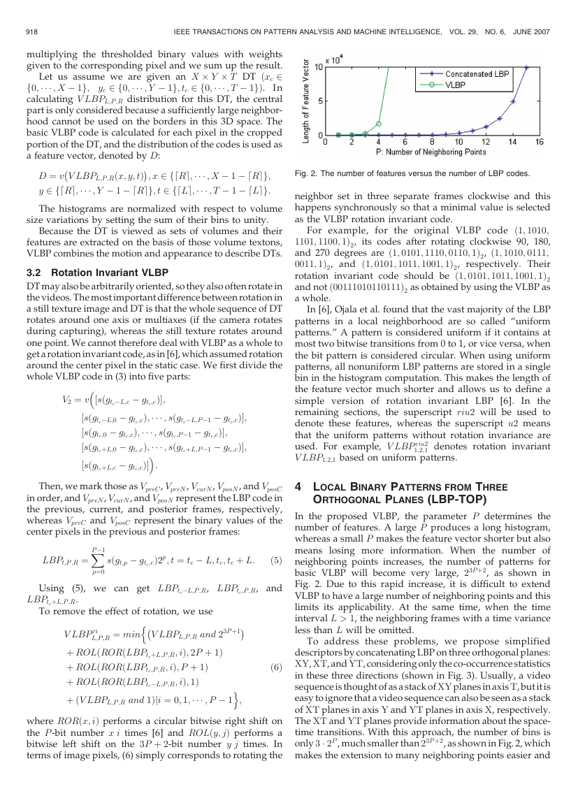
Fig. 3. Three planes in DT to extract neighboring points.
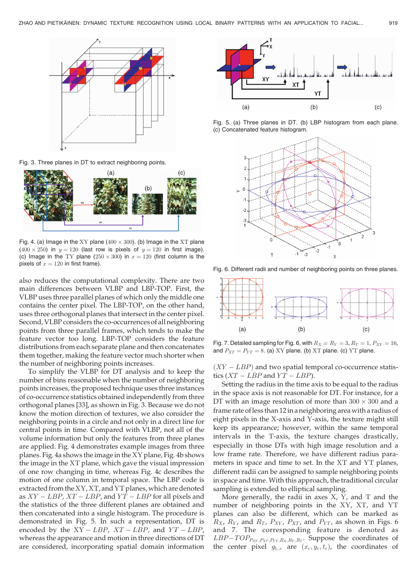
Fig. 4. (a) Image in the XY plane (400 � 300). (b) Image in the XT plane
(400 � 250) in y ¼ 120 (last row is pixels of y ¼ 120 in first image).
(c) Image in the TY plane (250 � 300) in x ¼ 120 (first column is the
pixels of x ¼ 120 in first frame).
also reduces the computational complexity. There are two
main differences between VLBP and LBP-TOP. First, the
VLBP uses three parallel planes of which only the middle one
contains the center pixel. The LBP-TOP, on the other hand,
uses three orthogonal planes that intersect in the center pixel.
Second, VLBP considers the co-occurrences of all neighboring
points from three parallel frames, which tends to make the
feature vector too long. LBP-TOP considers the feature
distributions from each separate plane and then concatenates
them together, making the feature vector much shorter when
the number of neighboring points increases.
To simplify the VLBP for DT analysis and to keep the
number of bins reasonable when the number of neighboring
points increases, the proposed technique uses three instances
of co-occurrence statistics obtained independently from three
orthogonal planes [33], as shown in Fig. 3. Because we do not
know the motion direction of textures, we also consider the
neighboring points in a circle and not only in a direct line for
central points in time. Compared with VLBP, not all of the
volume information but only the features from three planes
are applied. Fig. 4 demonstrates example images from three
planes. Fig. 4a shows the image in the XY plane, Fig. 4b shows
the image in the XT plane, which gave the visual impression
of one row changing in time, whereas Fig. 4c describes the
motion of one column in temporal space. The LBP code is
extracted from the XY, XT, and YT planes, which are denoted
as XY � LBP , XT � LBP , and Y T � LBP for all pixels and
the statistics of the three different planes are obtained and
then concatenated into a single histogram. The procedure is
demonstrated in Fig. 5. In such a representation, DT is
encoded by the XY � LBP , XT � LBP , and Y T � LBP ,
whereas the appearance and motion in three directions of DT
are considered, incorporating spatial domain information
Fig. 6. Different radii and number of neighboring points on three planes.
Fig. 7. Detailed sampling for Fig. 6, with RX ¼ RY ¼ 3, RT ¼ 1, PXY ¼ 16,
and PXT ¼ PY T ¼ 8. (a) XY plane. (b) XT plane. (c) YT plane.
ðXY � LBPÞ and two spatial temporal co-occurrence statis-
tics (XT � LBP and Y T � LBP ).
Setting the radius in the time axis to be equal to the radius
in the space axis is not reasonable for DT. For instance, for a
DT with an image resolution of more than 300 � 300 and a
frame rate of less than 12 in a neighboring area with a radius of
eight pixels in the X-axis and Y-axis, the texture might still
keep its appearance; however, within the same temporal
intervals in the T-axis, the texture changes drastically,
especially in those DTs with high image resolution and a
low frame rate. Therefore, we have different radius para-
meters in space and time to set. In the XT and YT planes,
different radii can be assigned to sample neighboring points
in space and time. With this approach, the traditional circular
sampling is extended to elliptical sampling.
More generally, the radii in axes X, Y, and T and the
number of neighboring points in the XY, XT, and YT
planes can also be different, which can be marked as
RX, RY , and RT , PXY , PXT , and PY T , as shown in Figs. 6
and 7. The corresponding feature is denoted as
LBP �T OPPXY ;PXT ;PY T ;RX;RY ;RT . Suppose the coordinates of
the center pixel gtc;c are ðxc; yc; tcÞ,
the coordinates of
�
920
IEEE TRANSACTIONS ON PATTERN ANALYSIS AND MACHINE INTELLIGENCE, VOL. 29, NO. 6,
JUNE 2007
the coordinates of
gXY ;p are given by ðxc � RX sinð2�p=PXY Þ; yc þ RY cos
ð2�p=PXY Þ; tcÞ,
gXT ;p are given
by ðxc � RX sinð2�p=PXTÞ; yc; tc � RT cosð2�p=PXTÞÞ, and the
coordinates of gY T ;p ðxc; yc � RY cosð2�p=PY TÞ; tc � RT sin
ð2�p=PY TÞÞ. This is different
from the ordinary LBP
the
widely used in many papers and it extends
definition of LBP.
Let us assume we are given an X � Y � T DT ðxc 2
f0;��� ; X � 1g; yc 2 f0;��� ; Y � 1g; tc 2 f0;��� ; T � 1gÞ. In
calculating LBP � T OPPXY ;PXT ;PY T ;RX;RY ;RT distribution for
this DT, the central part is only considered because a
sufficiently large neighborhood cannot be used on the
borders in this 3D space.
X
�
A histogram of the DT can be defined as
I fjðx; y; tÞ ¼ i
Hi;j ¼
i ¼ 0;��� ; nj � 1; j ¼ 0; 1; 2
;
x;y;t
in which nj is the number of different labels produced by the
LBP operator in the jth planeðj ¼ 0 : XY ; 1 : XT and 2 : Y TÞ,
fiðx; y; tÞ expresses the LBP code of central pixel ðx; y; tÞ in the
jth plane and IfAg ¼ 1; if A is true;
0; if A is false:
�
When the DTs to be compared are of different spatial and
temporal sizes, the histograms must be normalized to get a
coherent description:
Ni;j ¼
Hi;jP
nj�1
k¼0 Hk;j
:
ð8Þ
In this histogram, a description of DT is effectively
obtained based on LBP from three different planes. The
labels from the XY plane contain information about the
appearance, and, in the labels from the XT and YT planes,
co-occurrence statistics of motion in horizontal and vertical
directions are included. These three histograms are con-
catenated to build a global description of DT with the
spatial and temporal features.
5 LOCAL DESCRIPTORS FOR FACIAL IMAGE
ANALYSIS
Local texture descriptors have gained increasing attention in
facial image analysis due to their robustness to challenges
such as pose and illumination changes. Recently, Ahonen
et al. proposed a novel facial representation for face recogni-
tion from static images based on LBP features [34], [35]. In this
approach, the face image is divided into several regions
(blocks) from which the LBP features are extracted and
concatenated into an enhanced feature vector. This approach
is proving to be a growing success. It has been adopted and
further developed by many research groups and has been
successfully used for face recognition, face detection, and
facial expression recognition [35]. All of these have applied
LBP-based descriptors only for static images, that is, they do
not utilize temporal information as proposed in this paper.
In this section, a block-based approach for combining
pixel-level, region-level, and temporal
information is
proposed. Facial expression recognition is used as a case
study, but a similar approach could be used for recognizing
other specific dynamic events such as faces from video, for
example. The goal of facial expression recognition is to
determine the emotional state of the face, for example,
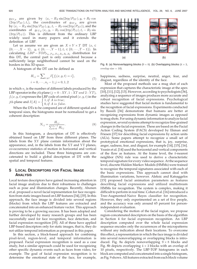
Fig. 8. (a) Nonoverlapping blocks (9 � 8). (b) Overlapping blocks (4 � 3,
overlap size ¼ 10).
ð7Þ
happiness, sadness, surprise, neutral, anger,
disgust, regardless of the identity of the face.
fear, and
Most of the proposed methods use a mug shot of each
expression that captures the characteristic image at the apex
[10], [11], [12], [13]. However, according to psychologists [36],
analyzing a sequence of images produces more accurate and
robust recognition of facial expressions. Psychological
studies have suggested that facial motion is fundamental to
the recognition of facial expressions. Experiments conducted
by Bassili [36] demonstrate that humans are better at
recognizing expressions from dynamic images as opposed
to mug shots. For using dynamic information to analyze facial
expression, several systems attempt to recognize fine-grained
changes in the facial expression. These are based on the Facial
Action Coding System (FACS) developed by Ekman and
Friesen [37] for describing facial expressions by action units
(AUs). Some papers attempt to recognize a small set of
prototypical emotional expressions, that is,
joy, surprise,
anger, sadness, fear, and disgust, for example [14], [15], [16].
Yeasin et al. [14] used the horizontal and vertical components
of the flow as features. At the frame level, the k-nearest
neighbor (NN) rule was used to derive a characteristic
temporal signature for every video sequence. At the sequence
level, discrete Hidden Markov Models (HMMs) were trained
to recognize the temporal signatures associated with each of
the basic expressions. This approach cannot deal with
illumination variations, however. Aleksic and Katsaggelos
[15] proposed facial animation parameters as features
describing facial expressions and utilized multistream
HMMs for recognition. The system is complex, making it
difficult to perform in real time. Cohen et al. [16] introduced a
Tree-Augmented-Naive Bayes classifier for recognition.
However, they only experimented on a set of five people,
and the accuracy was only around 65 percent for person-
independent evaluation.
Considering the motion of the facial region, we propose
region-concatenated descriptors on the basis of the algorithm
in Section 4 for facial expression recognition. An LBP
description computed over the whole facial expression
sequence encodes only the occurrences of the micropatterns
without any indication about their locations. To overcome
this effect, a representation in which the face image is divided
into several nonoverlapping or overlapping blocks is intro-
duced. Fig. 8a depicts nonoverlapping 9 � 8 blocks and
Fig. 8b depicts overlapping 4 � 3 blocks with an overlap of
10 pixels, respectively. The LBP-TOP histograms in each
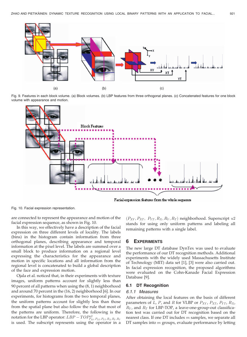
block are computed and concatenated into a single histogram,
as Fig. 9 shows. All features extracted from each block volume
�
ZHAO AND PIETIKA¨ INEN: DYNAMIC TEXTURE RECOGNITION USING LOCAL BINARY PATTERNS WITH AN APPLICATION TO FACIAL...
921
Fig. 9. Features in each block volume. (a) Block volumes. (b) LBP features from three orthogonal planes. (c) Concatenated features for one block
volume with appearance and motion.
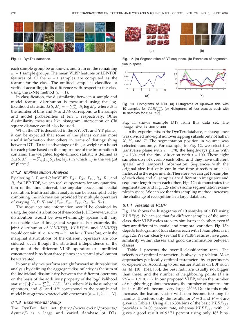
Fig. 10. Facial expression representation.
are connected to represent the appearance and motion of the
facial expression sequence, as shown in Fig. 10.
In this way, we effectively have a description of the facial
expression on three different levels of locality. The labels
(bins) in the histogram contain information from three
orthogonal planes, describing appearance and temporal
information at the pixel level. The labels are summed over a
small block to produce information on a regional level
expressing the characteristics for the appearance and
motion in specific locations and all information from the
regional level is concatenated to build a global description
of the face and expression motion.
Ojala et al. noticed that, in their experiments with texture
images, uniform patterns account for slightly less than
90 percent of all patterns when using the (8, 1) neighborhood
and around 70 percent in the (16, 2) neighborhood [6]. In our
experiments, for histograms from the two temporal planes,
the uniform patterns account for slightly less than those
from the spatial plane but also follow the rule that most of
the patterns are uniform. Therefore, the following is the
notation for the LBP operator: LBP � T OP u2
PXY ;PXT ;PY T ;RX;RY ;RT
is used. The subscript represents using the operator in a
ðPXY ; PXT ; PY T ; RX; RY ; RTÞ neighborhood. Superscript u2
stands for using only uniform patterns and labeling all
remaining patterns with a single label.
6 EXPERIMENTS
The new large DT database DynTex was used to evaluate
the performance of our DT recognition methods. Additional
experiments with the widely used Massachusetts Institute
of Technology (MIT) data set [1], [3] were also carried out.
In facial expression recognition, the proposed algorithms
were evaluated on the Cohn-Kanade Facial Expression
Database [9].
6.1 DT Recognition
6.1.1 Measures
After obtaining the local features on the basis of different
parameters of L, P , and R for VLBP or PXY , PXT , PY T , RX,
RY , and RT for LBP-TOP, a leave-one-group-out classifica-
tion test was carried out for DT recognition based on the
nearest class. If one DT includes m samples, we separate all
DT samples into m groups, evaluate performance by letting
�
922
IEEE TRANSACTIONS ON PATTERN ANALYSIS AND MACHINE INTELLIGENCE, VOL. 29, NO. 6,
JUNE 2007
Fig. 11. DynTex database.
Fig. 12. (a) Segmentation of DT sequence. (b) Examples of segmenta-
tion in space.
each sample group be unknown, and train on the remaining
m � 1 sample groups. The mean VLBP features or LBP-TOP
features of all the m � 1 samples are computed as the
feature for the class. The omitted sample is classified or
verified according to its difference with respect to the class
using the k-NN method ðk ¼ 1Þ.
P
In classification, the dissimilarity between a sample and
feature distribution is measured using the log-
model
likelihood statistic: LðS; MÞ ¼ �
B
b¼1 Sb log Mb, where B is
the number of bins and Sb and Mb correspond to the sample
and model probabilities at bin b, respectively. Other
dissimilarity measures like histogram intersection or Chi
square distance could also be used.
When the DT is described in the XY, XT, and YT planes,
it can be expected that some of the planes contain more
useful information than others in terms of distinguishing
between DTs. To take advantage of this, a weight can be set
for each plane based on the importance of the information it
contains. The weighted log-likelihood statistic is defined as
i;jðwjSj;i log Mj;iÞ in which wj is the weight
LwðS; MÞ ¼ �
of plane j.
P
6.1.2 Multiresolution Analysis
By altering L, P , and R for VLBP, PXY , PXT , PY T , RX, RY , and
RT for LBP-TOP, we can realize operators for any quantiza-
tion of the time interval, the angular space, and spatial
resolution. Multiresolution analysis can be accomplished by
combining the information provided by multiple operators
of varying ðL; P ; RÞ and ðPXY ; PXT ; PY T ; RX; RY ; RTÞ.
The most accurate information would be obtained by
using the joint distribution of these codes [6]. However, such a
distribution would be overwhelmingly sparse with any
reasonable size of image and sequence. For example, the
joint distribution of V LBP riu2
2;4;1, and V LBP riu2
2;8;1
would contain 16 � 16 � 28 ¼ 7; 168 bins. Therefore, only the
marginal distributions of the different operators are con-
sidered, even though the statistical independence of the
outputs of the different VLBP operators or simplified
concatenated bins from three planes at a central pixel cannot
be warranted.
1;4;1, V LBP riu2
In our study, we perform straightforward multiresolution
analysis by defining the aggregate dissimilarity as the sum of
P
the individual dissimilarity between the different operators
on the basis of the additivity property of the log-likelihood
statistic [6]: LN ¼
n¼1 LðSn; M nÞ, where N is the number of
operators, and Sn and Mn correspond to the sample and
model histograms extracted with operator nðn ¼ 1; 2;��� ; NÞ.
N
6.1.3 Experimental Setup
The DynTex data set
dyntex/)
(http://www.cwi.nl/projects/
is a large and varied database of DTs.
Fig. 13. Histograms of DTs. (a) Histograms of up-down tide with
10 samples for V LBP riu2
2;2;1. (b) Histograms of four classes each with
10 samples for V LBP riu2
2;2;1.
Fig. 11 shows example DTs from this data set. The
image size is 400 � 300.
In the experiments on the DynTex database, each sequence
was divided into eight nonoverlapping subsets but not half in
X, Y , and T . The segmentation position in volume was
selected randomly. For example, in Fig. 12, we select the
transverse plane with x ¼ 170, the lengthways plane with
y ¼ 130, and the time direction with t ¼ 100. These eight
samples do not overlap each other and they have different
spatial and temporal
information. Sequences with the
original size but only cut in the time direction are also
included in the experiments. Therefore, we can get 10 samples
of each class and all samples are different in image size and
sequence length from each other. Fig. 12a demonstrates the
segmentation and Fig. 12b shows some segmentation exam-
ples in space. We can see that this sampling method increases
the challenge of recognition in a large database.
6.1.4 Results of VLBP
Fig. 13a shows the histograms of 10 samples of a DT using
V LBP riu2
2;2;1. We can see that for different samples of the same
class, their VLBP codes are very similar to each other, even if
they are different in spatial and temporal variation. Fig. 13b
depicts histograms of four classes each with 10 samples, as in
Fig. 12a. We can clearly see that the VLBP features have good
similarity within classes and good discrimination between
classes.
Table 1 presents the overall classification rates. The
selection of optimal parameters is always a problem. Most
approaches get locally optimal parameters by experiments
or experience. According to our earlier studies on LBP such
as [6], [10], [34], [35], the best radii are usually not bigger
than three, and the number of neighboring points ðPÞ is
2nðn ¼ 1; 2; 3;���Þ. In our proposed VLBP, when the number
of neighboring points increases, the number of patterns for
basic VLBP will become very large: 23Pþ2. Due to this rapid
increase, the feature vector will soon become too long to
handle. Therefore, only the results for P ¼ 2 and P ¼ 4 are
given in Table 1. Using all 16,384 bins of the basic V LBP2;4;1
provides a 94.00 percent rate, whereas V LBP2;4;1 with u2
gives a good result of 93.71 percent using only 185 bins.
�



 2023年江西萍乡中考道德与法治真题及答案.doc
 2012年重庆南川中考生物真题及答案.doc
 2013年江西师范大学地理学综合及文艺理论基础考研真题.doc
 2020年四川甘孜小升初语文真题及答案I卷.doc
 2020年注册岩土工程师专业基础考试真题及答案.doc
 2023-2024学年福建省厦门市九年级上学期数学月考试题及答案.doc
 2021-2022学年辽宁省沈阳市大东区九年级上学期语文期末试题及答案.doc
 2022-2023学年北京东城区初三第一学期物理期末试卷及答案.doc
 2018上半年江西教师资格初中地理学科知识与教学能力真题及答案.doc
 2012年河北国家公务员申论考试真题及答案-省级.doc
 2020-2021学年江苏省扬州市江都区邵樊片九年级上学期数学第一次质量检测试题及答案.doc
 2022下半年黑龙江教师资格证中学综合素质真题及答案.doc