Analysis and Improvement of the Consistency of
Extended Kalman Filter based SLAM
Guoquan P. Huang, Anastasios I. Mourikis and Stergios I. Roumeliotis
Dept. of Computer Science and Engineering, University of Minnesota, Minneapolis, MN 55455
email:{ghuang|mourikis|stergios}@cs.umn.edu
Abstract— In this work, we study the inconsistency of EKF-
based SLAM from the perspective of observability. We analyti-
cally prove that when the Jacobians of the state and measurement
models are evaluated at the latest state estimates during every
time step, the linearized error-state system model of the EKF-
based SLAM has observable subspace of dimension higher than
that of the actual, nonlinear, SLAM system. As a result, the
covariance estimates of the EKF undergo reduction in directions
of the state space where no information is available, which is
a primary cause of inconsistency. To address this issue, a new
“First Estimates Jacobian” (FEJ) EKF is proposed, which is
shown to perform better in terms of consistency. In the FEJ-
EKF, the filter Jacobians are calculated using the first-ever
available estimates for each state variable, which insures that
the observable subspace of the error-state system model is of
the same dimension as that of the underlying nonlinear SLAM
system. The theoretical analysis is validated through extensive
simulations.
I. INTRODUCTION
For autonomous vehicles exploring unknown environments,
the ability to perform simultaneous localization and mapping
(SLAM) is essential. Among the numerous algorithms devel-
oped thus far for the SLAM problem, the extended Kalman
filter (EKF) remains one of the most popular ones, and has
been used in several practical applications. In this work, we
address the consistency issue of the EKF-SLAM algorithm,
which has recently received considerable attention [1]–[5]. As
defined in [6], a state estimator is consistent if the estimation
errors (i) are zero-mean, and (ii) have covariance matrix
smaller or equal to the one calculated by the filter. Consistency
is one of the primary criteria for evaluating the performance of
any estimator; if an estimator is inconsistent, then the accuracy
of the produced state estimates is unknown, which in turn
makes the estimator unreliable.
Since SLAM is a nonlinear estimation problem, no provably
consistent estimator can be constructed for it. The consistency
of every estimator has to be evaluated experimentally. In
particular for the standard EKF-SLAM algorithm, there exists
significant empirical evidence showing that the computed state
estimates tend to be inconsistent. The first work to draw
attention to this issue was that of Julier and Uhlmann [3].
Specifically, in [3] it was observed that when a stationary robot
measures the relative position of a new landmark multiple
times, the estimated variance of the robot’s orientation be-
comes smaller. Since the observation of a previously unseen
feature does not provide any information about the robot’s
state, this reduction is “artificial,” and leads to inconsistency.
Bailey et al. [2] examined several symptoms of the inconsis-
tency of the standard EKF algorithm, and argued, based on
simulation results, that the uncertainty in the robot orientation
is the main cause of the inconsistency of EKF-SLAM. The
work of [5] further confirmed the empirical findings in [2],
and argued by example that in EKF-SLAM the inconsistency is
always in the form of overconfident estimates (i.e., computed
covariances smaller than the actual ones).
The aforementioned works have described several symp-
toms of inconsistency that appear in the standard EKF-SLAM.
However, they have not conducted a detailed analysis into the
exact cause of the inconsistency (with the exception of [3]
for the special case of a stationary robot). In this paper,
we investigate in depth one of the fundamental causes of
inconsistency. In particular, we revisit this problem from a new
perspective, i.e., by analyzing the observability properties of
the filter’s error-state system model. The main contributions
of this work are the following:
• Through an observability analysis, we prove that the stan-
dard EKF-SLAM employs an error-state system model
that has an unobservable subspace of dimension two, even
though the underlying nonlinear system model has three
unobservable degrees of freedom (corresponding to the
position and orientation of the global reference frame).
This is a primary cause of filter inconsistency.
• We propose a new algorithm,
termed First Estimates
Jacobian (FEJ)-EKF, which improves the estimator’s con-
sistency during SLAM. Specifically, we show analytically
that when the EKF Jacobians are computed using the first-
ever available estimates for each of the state variables, the
error-state model has the same observability properties
as the underlying nonlinear model. As a result of these
properties, the new FEJ-EKF outperforms, in terms of
accuracy and consistency, alternative approaches to this
problem [1].
II. SLAM OBSERVABILITY ANALYSIS
The observability properties of SLAM have been studied
in few only cases in the literature. In particular, [7], [8]
investigated the observability of a simple linear time invariant
(LTI) SLAM system, and showed that
is unobservable.
On the other hand, in [9] the observability of the nonlinear
SLAM system was studied, using the nonlinear observability
rank condition developed by Hermann and Krener [10]. This
work proved that the underlying, nonlinear, SLAM system is
unobservable, with three unobservable degrees of freedom.
However, to the best of our knowledge, an analysis of the
observability properties of the EKF’s linearized error-state
system model does not exist to date. As shown in this paper,
it
�
these properties play a significant role in determining the
consistency of the filter.
In the following, after presenting the equations of the stan-
dard EKF-SLAM formulation, we compare its observability
properties with those of the underlying nonlinear system, and
use this analysis to draw conclusions about the consistency
of the filter. To preserve the clarity of the presentation, in
this section we consider the case where a single landmark is
included in the state vector. However, the conclusions drawn
in this case can be readily extended to the general case of
multiple landmarks. We note that, due to space limitations,
some intermediate steps of the derivations have been omitted;
the interested reader is referred to [11] for details.
A. Standard EKF-SLAM
In the standard formulation of SLAM,
the state vector
comprises the robot pose and the landmarks’ positions in the
global frame. Thus, at time-step k the state vector is given by
T =
T
xk =
pT
Rk
φRk pT
(1)
L
φRk]T denotes the robot pose (position
xT
Rk
pT
L
where xRk = [pT
Rk
and orientation), and pL is the landmark position.
1) EKF Propagation: In the propagation step, the robot’s
odometry measurements are processed to obtain an estimate of
the pose change between two consecutive time steps, and then
employed in the EKF to propagate the robot state estimate.
On the other hand, since the landmark is static, its estimate
does not change with the incorporation of a new odometry
measurement. The EKF propagation equations are given by:1
ˆpRk+1|k =ˆpRk|k + C( ˆφRk|k)Rk ˆpRk+1
ˆφRk+1|k = ˆφRk|k + Rk ˆφRk+1
ˆpLk+1|k =ˆpLk|k
(2)
(3)
(4)
where C(·) denotes the 2× 2 rotation matrix, and Rk ˆxRk+1 =
Rk ˆφRk+1]T is the odometry-based estimate of
[Rk ˆpT
the robot’s motion between time-steps k and k + 1. This
estimate is corrupted by zero-mean, white Gaussian noise
wk = RkxRk+1 − Rk ˆxRk+1, with covariance matrix Qk.
In addition to the state propagation equations, the linearized
error-state propagation equation is necessary for the EKF. This
is given by:
Rk+1
˜xk+1|k =
ΦRk
02×3
03×2
I2
˜xRk|k
˜xLk|k
+
GRk
02×2
Φk˜xk|k + Gkwk
(5)
where ΦRk and GRk are obtained from the state propagation
equations (2)-(3) as [11]:
ΦRk =
I2
01×2
JC( ˆφRk|k)Rk ˆpRk+1
1
(6)
1Throughout this paper the subscript |j refers to the estimate of a quantity
at time-step , after all measurements up to time-step j have been processed.
ˆx is used to denote the estimate of a random variable x, while ˜x = x − ˆx is
the error in this estimate. 0m×n and 1m×n denote m× n matrices of zeros
and ones, respectively, while In is the n × n identity matrix. Finally, we use
the concatenated forms sφ and cφ to denote the sin φ and cos φ functions,
respectively.
ˆpRk+1|k − ˆpRk|k
≡
1
J
I2
01×2
C( ˆφRk|k) 02×1
1
01×2
GRk =
0 −1
1
0
.
(7)
(8)
where J
It is important to point out that the form of the propagation
equations presented above is general, and holds for any robot
kinematic model (e.g., unicycle, bicycle, or Ackerman model).
For example, if the unicycle model is used, and we employ
the approximation that the velocity and heading are constant
during each propagation interval, we obtain Rk ˆxRk+1 =
[vmk δt 0 ωmk δt]T , where vmk and ωmk are the linear and
rotational velocity measurements, respectively, and δt is the
sampling period. Substitution in (2)-(3) yields the familiar
robot pose propagation equations:
ˆpRk+1|k =ˆpRk|k +
ˆφRk+1|k = ˆφRk|k + ωmk δt
vmk δtc( ˆφRk|k)
vmk δts( ˆφRk|k)
(9)
(10)
Similarly, the commonly used expressions for the matrices
ΦRk and GRk can be derived from (5), (6) and (8) (cf. [11]).
2) EKF Update: The measurement used for updates in the
EKF is a function of the relative position of the landmark with
respect to the robot:
CT (φRk)(pLk − pRk)
zk = h(xk) + vk = h
+ vk
(11)
where vk is zero-mean Gaussian measurement noise with co-
variance Rk. In this work, we allow h to be any 2-dimensional
measurement function, as long as it is invertible (i.e., as long
as we can fully determine an estimate of the robot-relative
landmark position from zk). For instance, this is the case when
zk is a direct measurement of relative position, a pair of range
and bearing measurements, two bearing measurements from
the cameras of a stereo pair, etc. Generally, the measurement
function is nonlinear, and hence it is linearized for use in the
EKF. The linearized measurement-error equation is given by
˜zk
HRk HLk
˜xRk|k−1
˜xLk|k−1
+ vk
(12)
−I2 −J(ˆpLk|k−1 − ˆpRk|k−1)
where HRk and HLk are the Jacobians of h with respect
to the robot pose and the landmark position, respectively,
evaluated at the state estimate ˆxk|k−1. Using the chain rule
of differentiation, these are computed as:
HRk =(∇hk)CT ( ˆφRk|k−1)
(13)
HLk =(∇hk)CT ( ˆφRk|k−1)
(14)
where ∇hk denotes the Jacobian of h with respect to the
robot-relative landmark position (i.e., with respect to the vector
RkpL = CT (φRk)(pL−pRk)), evaluated at the state estimate
ˆxk|k−1.
wk
Hk˜xk|k−1 + vk
�
B. Nonlinear Observability Analysis for SLAM
Before studying the observability properties of the EKF
system model, we conduct the observability analysis for the
underlying continuous-time nonlinear SLAM system. By com-
paring the properties of the actual, nonlinear, system with
those of the EKF system model, we will be able to identify a
fundamental shortcoming of the standard EKF formulation,
which leads to filter inconsistency. The nonlinear observ-
ability analysis is based on the observability rank condition
introduced in [10]. Specifically, Theorem 3.11 in [10] proves
that “if a nonlinear system is locally weakly observable, the
observability rank condition is satisfied generically”. We here
show that the SLAM system does not satisfy the observability
rank condition, and thus it is not locally weakly observable
nor locally observable.
sφ(t)
ω(t)
v(t) +
For the continuous-time analysis we employ a unicycle
kinematic model, and a relative-position measurement model,
although identical conclusions can be reached if different
models are used [9]. The system model in continuous-time
form is given by ˙xR(t)
˙yR(t)
˙φR(t)
˙xL(t)
˙yL(t)
⇒ ˙x(t) =f1v(t) + f2ω(t)
=
cφ(t)
T is the control input, consisting of linear
where u
and rotational velocity. The continuous-time relative-position
measurement model is described by the expressions:
z(t) = CT (φ(t))(pL − pR(t))
0
0
1
0
0
v ω
(15)
0
0
0
cφ(t)(xL(t) − xR(t)) + sφ(t)(yL(t) − yR(t))
−sφ(t)(xL(t) − xR(t)) + cφ(t)(yL(t) − yR(t))
h1(x)
h2(x)
(16)
=
=
The observability analysis for the system model described
in (15) and (16) proceeds by first computing the space spanned
hi (for k ∈ N, j = 1, 2,
by all the kth order Lie derivatives Lk
i = 1, 2), which we denote by G. The space dG, spanned by
fj
the gradients of the elements of G is [11]:
dG = span
sφ −cφ −cφ(xL − xR) − sφ(yL − yR) −sφ
cφ
(17)
cφ
sφ(xL − xR) − cφ(yL − yR) −cφ −sφ
The matrix shown above is the “observability matrix” for the
nonlinear SLAM system under consideration. Clearly, the rank
of this matrix is two, and thus the system is unobservable.
Intuitively, this is a consequence of the fact that we cannot
gain absolute, but rather only relative state information from
the available measurements.
sφ
Even though the notion of an “unobservable subspace”
cannot be strictly defined for this system, by examining the
interpretation of the basis of dG⊥, which is the
physical
subspace orthogonal to dG, we will gain useful information
M
for our analysis in Section II-C. By inspection, we see that
one possible basis for the space dG⊥ is given by
1 0 −yR
0 1
xR
0 0
1
1 0 −yL
0 1
xL
= span
dG⊥ = span
n1 n2 n3
(18)
From the structure of the vectors n1 and n2 we see that
a change in the state by ∆x = αn1 + βn2, α, β ∈ R
corresponds to a “shifting” of the x − y plane by α units
along x, and by β units along y. Thus, if the robot and
landmark positions are shifted equally, the states x and x+∆x
will be indistinguishable given the measurements. To better
understand the physical meaning of n3, we consider the case
where the x− y plane is rotated by a small angle δφ. Rotating
the coordinate system transforms any point x = [x y]T to a
point x = [x y]T , given by:
x
y
x
y
1 −δφ
1
δφ
x
y
=
+ δφ
−y
x
x
y
= C(δφ)
where we have employed the small-angle approximations
c(δφ) 1 and s(δφ) δφ. Using this result, we see that
if the plane containing the robot and landmarks is rotated by
δφ, the SLAM state vector will change to
x
y
φ
x
x
R
R
R
L
L
xR
yR
φR
xL
xL
+ δφ
−yR
xR
1
−yL
xL
= x + δφn3
x =
(19)
which indicates that the vector n3 corresponds to a rotation of
the x − y plane. Since n3 ∈ dG⊥, this result shows that any
such rotation is unobservable, and will cause no change to the
measurements. The preceding analysis for the meaning of the
basis vectors of dG⊥ agrees with intuition, which dictates that
the global coordinates of the state vector in SLAM (rotation
and translation) are unobservable.
C. EKF-SLAM Observability Analysis
In the previous section, it was shown that the underlying
physical system in SLAM has three unobservable degrees of
freedom. Thus, when the EKF is used for state estimation in
SLAM, we would expect that the system model employed by
the EKF also shares this property. However, in this section we
show that this is not the case: the unobservable subspace of the
linearized error-state model in the standard EKF is generally
of dimension only 2.
Since the linearized error-state model for EKF-SLAM is
time-varying, we employ the local observability matrix [12] to
perform the observability analysis. Specifically, for the EKF-
SLAM system considered in this work (cf. (5) and (12)), the
local observability matrix for the time interval between time-
steps k and k + m is defined as:
Hk
Hk+1Φk
...
Hk+mΦk+m−1 ··· Φk
(20)
�
which can be expanded by substituting the matrices Φi and
Hi (cf. (5) and (12), respectively), to yield:
HLk
HLk+1
...
HRk
...
HRk+1ΦRk
M =
(21)
HRk+mΦRk+m−1 ··· ΦRk HLk+m
= Diag(HLk ,··· , HLk+m)×
HRk
H−1
Lk
H−1
Lk+1HRk+1ΦRk
I2
I2
...
I2
H−1
Lk+m
HRk+mΦRk+m−1 ··· ΦRk
...
(22)
N
The system is locally observable over the time period from
k to k + m if and only if the local observability matrix
M is full-rank. Since the matrix Diag(HLk ,··· , HLk+m)
is nonsingular, it becomes clear that rank(M) = rank(N),
and moreover, the matrices M and N have the same right
nullspace. Therefore, studying the rank and nullspace of N is
equivalent to studying those of M.
1) Ideal EKF-SLAM: Before considering the rank of the
matrix M, which is constructed using the estimated values of
the state in the filter Jacobians, it is interesting to study the
observability properties of the “oracle”, or “ideal” EKF (i.e.,
the filter whose Jacobians are evaluated using the true values
of the state variables). In the following, all matrices evaluated
using the true state values are denoted by the symbol “ ˘ ”.
We start by noting that (cf. (7)):
J
˘ΦRk+1
˘ΦRk =
I2
01×2
pRk+2 − pRk
Based on this property, it is easy to show by induction that:
(23)
1
pRk+i − pRk
1
˘ΦRk+i−1
˘ΦRk+i−2 ··· ˘ΦRk =
J
I2
01×2
where i > 0. Using this result, and substituting for the
measurement Jacobians from (13) and (14), we can prove the
following useful identity:
˘H−1
Lk+i
=
˘HRk
which holds for all i > 0. N can now be written as
Lk
˘HRk+i
= ˘H−1
−I2 −J(pL − pRk)
˘ΦRk+i−1 ··· ˘ΦRk
=
−I2 −J(pL − pRk)
−I2 −J(pL − pRk)
...
−I2 −J(pL − pRk)
I2
I2
...
I2
...
Lk
Lk
˘H−1
˘HRk
˘H−1
˘HRk
...
˘H−1
˘HRk
Lk
˘N =
(24)
I2
I2
I2
Clearly, rank( ˘N) = 2 and thus the ideal EKF system model
is unobservable. Most importantly, however, it can be easily
verified that a basis for the right nullspace of ˘N (and thus
for the right nullspace of ˘M) is given by the vectors shown
in (18). Thus, the unobservable subspace of the ideal EKF
system model is identical to the space dG⊥, that contains the
unobservable directions of the nonlinear SLAM system. We
therefore see that if it was possible to evaluate the Jacobians
using the true state values, the linearized error-state model
employed in the EKF would have observability properties
similar to those of the actual, nonlinear SLAM system.
2) Standard EKF-SLAM: We now examine the observabil-
ity properties of the EKF when the Jacobians are evaluated
using the latest state estimates, which is the case in a real
implementation. We start by deriving an expression analogous
to that of (23). We obtain:
J
ˆpRk+2|k+1 − ˆpRk|k − ∆pRk+1
ΦRk+1ΦRk =
where ∆pRk+1 = ˆpRk+1|k+1 − ˆpRk+1|k is the correction in
the robot position due to the update at time-step k + 1. Using
induction, we can show that:
ΦRk+i−1ΦRk+i−2 ··· ΦRk =
I2
01×2
(25)
1
I2
01×2
1
where i > 0. Moreover, we obtain:
HRk+iΦRk+i−1 ··· ΦRk
I2 J
H−1
= −
Lk+i
J
ˆpLk+i|k+i−1 − ˆpRk|k +
ˆpRk+i|k+i−1 − ˆpRk|k −k+i−1
k+i−1
ˆpLk|k−1 − ˆpRk|k−1
−J
−J
ˆpLk+1|k − ˆpRk|k
ˆpLk+2|k+1 − ˆpRk|k + ∆pRk+1
k+i−1
ˆpLk+i|k+i−1 − ˆpRk|k +
−J
...
N =
−I2
−I2
−I2
...
−I2 −J
Using this result, we can write matrix N as:
j=k+1 ∆pRj
(26)
(27)
I2
I2
I2
...
I2
j=k+1 ∆pRj
j=k+1 ∆pRj
At this point, we note that the corrections of the robot position
at any given time step are generally nonzero, and additionally,
the landmark state estimates at different time instants are not
equal. Therefore, the third column of N will be, in general,
a vector with unequal elements, and hence rank(N) = 3.
We thus see that the linearized error-state model employed in
the standard EKF-SLAM has different observability properties
than the underlying nonlinear system. In particular, by process-
ing the measurements collected in the interval [k, k + m], the
EKF acquires information in 3 dimensions of the state space
(along the directions corresponding to the observable subspace
of the EKF). However, as the nonlinear observability analysis
of Section II-B shows, the measurements actually provide
information in only 2 directions of the state space. As a result,
the EKF gains “spurious information” along the unobservable
directions of the underlying nonlinear SLAM system, which
leads to inconsistency.
To probe further, we note that the basis of the right nullspace
of N is given by:
null(N) =
n1 n2
(28)
which, as explained in Section II-B corresponds to a shifting of
the x− y plane. It is interesting to point out that the “missing”
�
direction in the unobservable subspace of the EKF system
model is the one along the vector n3, which corresponds to a
rotation of the x−y plane. Therefore, we see that the filter will
gain “nonexistent” information about the robot’s orientation.
This will lead to an unjustified reduction in the uncertainty
of the robot’s orientation, which will, in turn, further reduce
the uncertainty in all the state variables. This agrees in some
respects with [2], [5], where it was argued that the orientation
uncertainty is the major cause of the filter’s inconsistency.
However, we point out that the root cause of the problem is the
fact that the Jacobians are evaluated at different linearization
points at every time step. This changes the dimension of
the observable subspace, and thus fundamentally alters the
properties of the estimation process.
An additional interesting point is that the covariance matrix
of the measurements does not appear in the observability
analysis of the filter. Therefore, even if this covariance matrix
is artificially inflated, the filter will retain the same observ-
ability properties (i.e., the same observable and unobservable
subspaces). This shows that no amount of covariance inflation
can result in correct observability properties. Similarly, even
if the Iterated EKF is employed for state estimation,
the
same, erroneous, observability properties will arise, since the
landmark position estimates will generally differ at different
time steps.
As a final remark, we note the “correct” observability
properties of the ideal EKF are attributed to the fact that (24)
holds, which is not the case for the standard EKF. When
condition (24) is met, it ensures that all the block rows of
the matrix N are identical, and leads to an unobservable
subspace of dimension three. Thus, (24) can be seen as a
sufficient condition that, when satisfied by the filter Jaco-
bians, ensures correct observability properties. Interestingly, as
shown in [11], (24) is equivalent to the condition derived in [3]
(cf. Theorem 1 therein), for the case where the robot remains
stationary. This indicates that
the Jacobian constraint (24)
derived based on the observability criterion is more general,
and encompasses the constraint of [3] as a special case.
III. FIRST-ESTIMATES JACOBIAN EKF SLAM
Careful observation of the matrix N in (27) reveals that it
is possible to obtain an EKF system model with an unobserv-
able subspace of dimension three, even if the Jacobians are
not evaluated at the true state values. For this purpose, the
following two changes are necessary.
1) Instead of computing the state-propagation Jacobian
matrix ΦRk as in (7), we employ the expression:
ˆpRk+1|k − ˆpRk|k−1
1
(29)
Φ
Rk
=
J
I2
01×2
The difference compared to (7) is that the robot position
estimate prior to updating, ˆpRk|k−1, is employed in this
computation instead of the updated estimate, ˆpRk|k.
2) In the evaluation of the measurement Jacobian matrix
HRk (cf. (13)) we always utilize the landmark estimate
from the first time the landmark was detected. Thus, if a
landmark was first seen at time-step , we compute the
measurement Jacobian with respect to the robot pose as:
H
−I2 −J(ˆpL| − ˆpRk|k−1)
=(∇hk)CT ( ˆφRk|k−1)
Rk
(30)
that
As a result of the above modifications, only the first esti-
mates of all landmark positions and all robot poses appear
in the Jacobians of the filter. This has as effect
the
observability matrix N of this new filter, which we term First-
Estimates Jacobian (FEJ)-EKF, assumes the form:
I2
I2
I2
...
I2
ˆpL| − ˆpRk|k−1
ˆpL| − ˆpRk|k−1
ˆpL| − ˆpRk|k−1
ˆpL| − ˆpRk|k−1
−I2 −J
−I2 −J
−I2 −J
...
−I2 −J
N =
...
This matrix is of rank 2, and thus the FEJ-EKF is based
on an error-state system model whose unobservable subspace
is of dimension 3. We stress that the FEJ-EKF estimator is
realizable “in the real world”, since it does not utilize any
knowledge of the true state. Interestingly, even though this
new filter does not use the latest available state estimates (and
thus utilizes Jacobians that are less accurate than those of the
standard EKF), it exhibits better consistency properties than
the standard EKF, as shown in the following section.
IV. SIMULATION RESULTS
A series of Monte-Carlo comparison studies were conducted
under various conditions, in order to validate the preceding
theoretical analysis and to demonstrate the capability of the
FEJ-EKF filter to improve the consistency of EKF-SLAM.
The metrics used to evaluate filter performance are: (i) the
RMS error, and (ii) the average normalized (state) estimation
error squared (NEES) [6]. Specifically, for the landmarks
we compute the average RMS and average NEES errors by
averaging the squared errors and the NEES, respectively, over
all Monte Carlo runs, all landmarks and all time steps. On the
other hand, for the robot pose we compute these error metrics
by averaging over all Monte Carlo runs for each time step
(cf. [11] for a more detailed description).
The RMS of estimation errors provide us with a concise
metric of the accuracy of a given estimator. On the other hand,
the NEES is a powerful metric for evaluating filter consistency.
Specifically, it is known that the NEES of an M-dimensional
Gaussian random variable follows a χ2 distribution with M
degrees of freedom. Therefore, if a certain filter is consistent,
we expect that the average NEES for the robot pose will be
close to 3 for all k, and that the average landmark NEES will
be close to 2. The larger the deviations of the NEES from these
values, the larger the inconsistency of the filter. By studying
both the RMS errors and NEES of all the filters, we obtain a
comprehensive picture of the estimators’ performance.
In all the simulation tests presented in this section, the
robot moves at a constant velocity of v = 0.25 m/sec, the
standard deviation of the velocity measurement noise is equal
to σv = 0.1v, while the rotational velocity measurements
are corrupted by noise with standard deviation σω = 1o/sec.
The robot records measurements of the relative position of
�
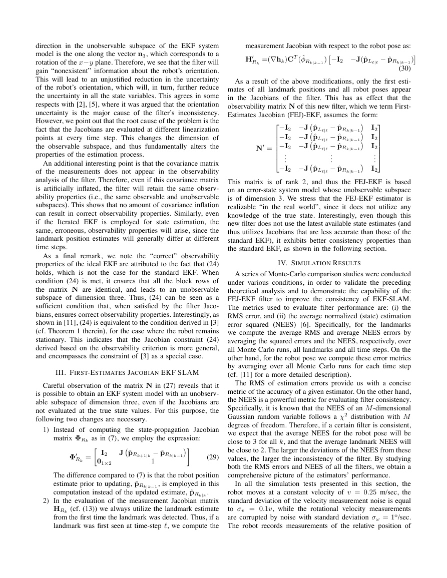
Fig. 1. Monte Carlo results for an exploration-SLAM scenario. (a) Average NEES of the robot pose errors (b) RMS errors for the robot pose (position and
orientation). In these plots, the solid lines correspond to the ideal EKF, the dashed lines to the FEJ-EKF, the solid lines with circles to the standard EKF, and
the dotted lines to the robocentric mapping algorithm of [4]. Note that the RMS errors of the ideal EKF, the FEJ-EKF, and the robo-centric SLAM algorithm
are almost identical, which makes the corresponding lines difficult to distinguish.
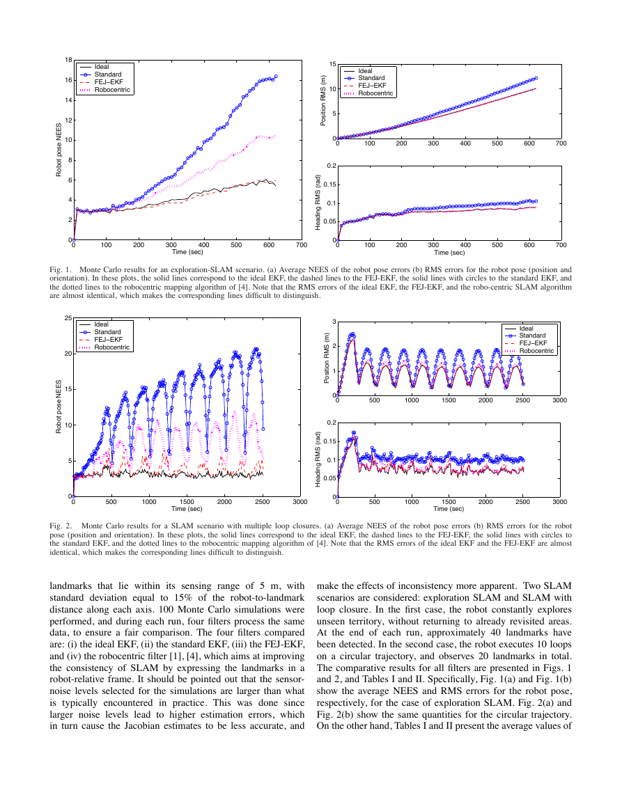
Fig. 2. Monte Carlo results for a SLAM scenario with multiple loop closures. (a) Average NEES of the robot pose errors (b) RMS errors for the robot
pose (position and orientation). In these plots, the solid lines correspond to the ideal EKF, the dashed lines to the FEJ-EKF, the solid lines with circles to
the standard EKF, and the dotted lines to the robocentric mapping algorithm of [4]. Note that the RMS errors of the ideal EKF and the FEJ-EKF are almost
identical, which makes the corresponding lines difficult to distinguish.
lie within its sensing range of 5 m, with
landmarks that
standard deviation equal
to 15% of the robot-to-landmark
distance along each axis. 100 Monte Carlo simulations were
performed, and during each run, four filters process the same
data, to ensure a fair comparison. The four filters compared
are: (i) the ideal EKF, (ii) the standard EKF, (iii) the FEJ-EKF,
and (iv) the robocentric filter [1], [4], which aims at improving
the consistency of SLAM by expressing the landmarks in a
robot-relative frame. It should be pointed out that the sensor-
noise levels selected for the simulations are larger than what
is typically encountered in practice. This was done since
larger noise levels lead to higher estimation errors, which
in turn cause the Jacobian estimates to be less accurate, and
make the effects of inconsistency more apparent. Two SLAM
scenarios are considered: exploration SLAM and SLAM with
loop closure. In the first case, the robot constantly explores
unseen territory, without returning to already revisited areas.
At the end of each run, approximately 40 landmarks have
been detected. In the second case, the robot executes 10 loops
on a circular trajectory, and observes 20 landmarks in total.
The comparative results for all filters are presented in Figs. 1
and 2, and Tables I and II. Specifically, Fig. 1(a) and Fig. 1(b)
show the average NEES and RMS errors for the robot pose,
respectively, for the case of exploration SLAM. Fig. 2(a) and
Fig. 2(b) show the same quantities for the circular trajectory.
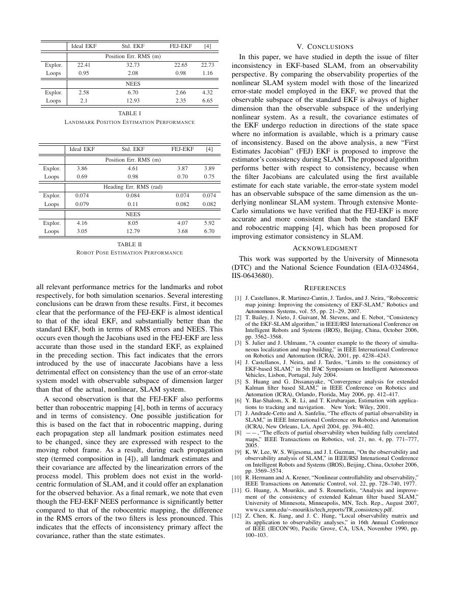
On the other hand, Tables I and II present the average values of
0100200300400500600700024681012141618Time (sec)Robot pose NEESIdealStandardFEJ−EKFRobocentric0100200300400500600700051015Position RMS (m)IdealStandardFEJ−EKFRobocentric010020030040050060070000.050.10.150.2Time (sec)Heading RMS (rad)0500100015002000250030000510152025Time (sec)Robot pose NEESIdealStandardFEJ−EKFRobocentric0500100015002000250030000123Position RMS (m)IdealStandardFEJ−EKFRobocentric05001000150020002500300000.050.10.150.2Time (sec)Heading RMS (rad)�
Ideal EKF
Std. EKF
FEJ-EKF
[4]
V. CONCLUSIONS
Explor.
Loops
Explor.
Loops
22.41
0.95
2.58
2.1
Position Err. RMS (m)
32.73
2.08
NEES
6.70
12.93
TABLE I
22.65
0.98
22.73
1.16
2.66
2.35
4.32
6.65
LANDMARK POSITION ESTIMATION PERFORMANCE
Ideal EKF
Std. EKF
FEJ-EKF
[4]
Explor.
Loops
Explor.
Loops
Explor.
Loops
3.86
0.69
0.074
0.079
4.16
3.05
Position Err. RMS (m)
4.61
0.98
Heading Err. RMS (rad)
0.084
0.11
NEES
8.05
12.79
TABLE II
3.87
0.70
3.89
0.75
0.074
0.082
0.074
0.082
4.07
3.68
5.92
6.70
ROBOT POSE ESTIMATION PERFORMANCE
all relevant performance metrics for the landmarks and robot
respectively, for both simulation scenarios. Several interesting
conclusions can be drawn from these results. First, it becomes
clear that the performance of the FEJ-EKF is almost identical
to that of the ideal EKF, and substantially better than the
standard EKF, both in terms of RMS errors and NEES. This
occurs even though the Jacobians used in the FEJ-EKF are less
accurate than those used in the standard EKF, as explained
in the preceding section. This fact indicates that the errors
introduced by the use of inaccurate Jacobians have a less
detrimental effect on consistency than the use of an error-state
system model with observable subspace of dimension larger
than that of the actual, nonlinear, SLAM system.
A second observation is that the FEJ-EKF also performs
better than robocentric mapping [4], both in terms of accuracy
and in terms of consistency. One possible justification for
this is based on the fact that in robocentric mapping, during
each propagation step all landmark position estimates need
to be changed, since they are expressed with respect to the
moving robot frame. As a result, during each propagation
step (termed composition in [4]), all landmark estimates and
their covariance are affected by the linearization errors of the
process model. This problem does not exist in the world-
centric formulation of SLAM, and it could offer an explanation
for the observed behavior. As a final remark, we note that even
though the FEJ-EKF NEES performance is significantly better
compared to that of the robocentric mapping, the difference
in the RMS errors of the two filters is less pronounced. This
indicates that the effects of inconsistency primary affect the
covariance, rather than the state estimates.
In this paper, we have studied in depth the issue of filter
inconsistency in EKF-based SLAM, from an observability
perspective. By comparing the observability properties of the
nonlinear SLAM system model with those of the linearized
error-state model employed in the EKF, we proved that the
observable subspace of the standard EKF is always of higher
dimension than the observable subspace of the underlying
nonlinear system. As a result, the covariance estimates of
the EKF undergo reduction in directions of the state space
where no information is available, which is a primary cause
of inconsistency. Based on the above analysis, a new “First
Estimates Jacobian” (FEJ) EKF is proposed to improve the
estimator’s consistency during SLAM. The proposed algorithm
performs better with respect to consistency, because when
the filter Jacobians are calculated using the first available
estimate for each state variable, the error-state system model
has an observable subspace of the same dimension as the un-
derlying nonlinear SLAM system. Through extensive Monte-
Carlo simulations we have verified that the FEJ-EKF is more
accurate and more consistent than both the standard EKF
and robocentric mapping [4], which has been proposed for
improving estimator consistency in SLAM.
ACKNOWLEDGMENT
This work was supported by the University of Minnesota
(DTC) and the National Science Foundation (EIA-0324864,
IIS-0643680).
REFERENCES
[1] J. Castellanos, R. Martinez-Cantin, J. Tardos, and J. Neira, “Robocentric
map joining: Improving the consistency of EKF-SLAM,” Robotics and
Autonomous Systems, vol. 55, pp. 21–29, 2007.
[2] T. Bailey, J. Nieto, J. Guivant, M. Stevens, and E. Nebot, “Consistency
of the EKF-SLAM algorithm,” in IEEE/RSJ International Conference on
Intelligent Robots and Systems (IROS), Beijing, China, October 2006,
pp. 3562–3568.
[3] S. Julier and J. Uhlmann, “A counter example to the theory of simulta-
neous localization and map building,” in IEEE International Conference
on Robotics and Automation (ICRA), 2001, pp. 4238–4243.
[4] J. Castellanos, J. Neira, and J. Tardos, “Limits to the consistency of
EKF-based SLAM,” in 5th IFAC Symposium on Intelligent Autonomous
Vehicles, Lisbon, Portugal, July 2004.
[5] S. Huang and G. Dissanayake, “Convergence analysis for extended
Kalman filter based SLAM,” in IEEE Conference on Robotics and
Automation (ICRA), Orlando, Florida, May 2006, pp. 412–417.
[6] Y. Bar-Shalom, X. R. Li, and T. Kirubarajan, Estimation with applica-
tions to tracking and navigation. New York: Wiley, 2001.
[7] J. Andrade-Cetto and A. Sanfeliu, “The effects of partial observability in
SLAM,” in IEEE International Conference on Robotics and Automation
(ICRA), New Orleans, LA, April 2004, pp. 394–402.
[8] ——, “The effects of partial observability when building fully correlated
maps,” IEEE Transactions on Robotics, vol. 21, no. 4, pp. 771–777,
2005.
[9] K. W. Lee, W. S. Wijesoma, and J. I. Guzman, “On the observability and
observability analysis of SLAM,” in IEEE/RSJ Intenational Conference
on Intelligent Robots and Systems (IROS), Beijing, China, October 2006,
pp. 3569–3574.
[10] R. Hermann and A. Krener, “Nonlinear controllability and observability,”
IEEE Transactions on Automatic Control, vol. 22, pp. 728–740, 1977.
[11] G. Huang, A. Mourikis, and S. Roumeliotis, “Analysis and improve-
ment of the consistency of extended Kalman filter based SLAM,”
University of Minnesota, Minneapolis, MN, Tech. Rep., August 2007,
www.cs.umn.edu/∼mourikis/tech reports/TR consistency.pdf.
[12] Z. Chen, K. Jiang, and J. C. Hung, “Local observability matrix and
its application to observability analyses,” in 16th Annual Conference
of IEEE (IECON’90), Pacific Grove, CA, USA, November 1990, pp.
100–103.
�


 2023年江西萍乡中考道德与法治真题及答案.doc
 2012年重庆南川中考生物真题及答案.doc
 2013年江西师范大学地理学综合及文艺理论基础考研真题.doc
 2020年四川甘孜小升初语文真题及答案I卷.doc
 2020年注册岩土工程师专业基础考试真题及答案.doc
 2023-2024学年福建省厦门市九年级上学期数学月考试题及答案.doc
 2021-2022学年辽宁省沈阳市大东区九年级上学期语文期末试题及答案.doc
 2022-2023学年北京东城区初三第一学期物理期末试卷及答案.doc
 2018上半年江西教师资格初中地理学科知识与教学能力真题及答案.doc
 2012年河北国家公务员申论考试真题及答案-省级.doc
 2020-2021学年江苏省扬州市江都区邵樊片九年级上学期数学第一次质量检测试题及答案.doc
 2022下半年黑龙江教师资格证中学综合素质真题及答案.doc