AdvancedCharacterPhysics.pdf

发布时间：2022-05-30 发布人：admin 分类：说明书资料大小：0.14M 资料格式：pdf 举报版权申诉

liuhua524-8018175-4744302542961894765.pdf-第1页.png

第1页 / 共16页

liuhua524-8018175-4744302542961894765.pdf-第2页.png

第2页 / 共16页

liuhua524-8018175-4744302542961894765.pdf-第3页.png

第3页 / 共16页

liuhua524-8018175-4744302542961894765.pdf-第4页.png

第4页 / 共16页

liuhua524-8018175-4744302542961894765.pdf-第5页.png

第5页 / 共16页

liuhua524-8018175-4744302542961894765.pdf-第6页.png

第6页 / 共16页

liuhua524-8018175-4744302542961894765.pdf-第7页.png

第7页 / 共16页

liuhua524-8018175-4744302542961894765.pdf-第8页.png

第8页 / 共16页

文本预览

Advanced Character Physics Página 1 de 16 Advanced Character Physics Thomas Jakobsen IO Interactive, Farvergade 2 DK-1463 Copenhagen K Denmark Email: tj@ioi.dk, www: www.ioi.dk/~tj Abstract This paper explains the basic elements of an approach to physically-based modeling which is well suited for interactive use. It is simple, fast, and quite stable, and in its basic version the method does not require knowledge of advanced mathematical subjects (although it is based on a solid mathematical foundation). It allows for simulation of both cloth; soft and rigid bodies; and even articulated or constrained bodies using both forward and inverse kinematics. The algorithms were developed for IO Interactive’s game Hitman: Codename 47. There, among other things, the physics system was responsible for the movement of cloth, plants, rigid bodies, and for making dead human bodies fall in unique ways depending on where they were hit, fully interacting with the environment (resulting in the press oxymoron “lifelike death animations”). The article also deals with subtleties like penetration test optimization and friction handling. 1 Introduction The use of physically-based modeling to produce nice-looking animation has been considered for some time and many of the existing techniques are fairly sophisticated. Different approaches have been proposed in the literature [Baraff, Mirtich, Witkin, and others] and much effort has been put into the construction of algorithms that are accurate and reliable. Actually, precise simulation methods for physics and dynamics have been known for quite some time from engineering. However, for games and interactive use, accuracy is really not the primary concern (although it’s certainly nice to have) – rather, here the important goals are believability (the programmer can cheat as much as he wants if the player still feels immersed) and speed of execution (only a certain time per frame will be allocated to the physics engine). In the case of physics simulation, the word believability also covers stability; a method is no good if objects seem to drift through obstacles or vibrate when they should be lying still, or if cloth particles tend to “blow up”. The methods demonstrated in this paper were created in an attempt to reach these goals. The algorithms were developed and implemented by the author for use in IO Interactive’s computer game Hitman: Codename 47, and have all been integrated in IO’s in-house game engine Glacier. The methods proved to be quite simple to implement (compared to other schemes at least) and have high performance. The algorithm is iterative such that, from a certain point, it can be stopped at any time. This gives us a very useful time/accuracy trade-off: If a small source of inaccuracy is accepted, the code can be allowed to run faster; this error margin can even be adjusted adaptively at run-time. In some cases, the method is as much as an order of magnitude faster than other existing methods. It also handles both collision and resting contact in the same framework and nicely copes with stacked boxes and other situations that stress a physics engine. In overview, the success of the method comes from the right combination of several techniques that all benefit from each other: A so-called Verlet integration scheme. file://C:\Documents%20and%20Settings\toni\Escritorio\Advanced%20Character%20... 24/02/2003

Advanced Character Physics Página 2 de 16 Handling collisions and penetrations by projection. A simple constraint solver using relaxation. A nice square root approximation that gives a solid speed-up. Modeling rigid bodies as particles with constraints. An optimized collision engine with the ability to calculate penetration depths. Each of the above subjects will be explained shortly. In writing this document, the author has tried to make it accessible to the widest possible audience without losing vital information necessary for implementation. This means that technical mathematical explanations and notions are kept to a minimum if not crucial to understanding the subject. The goal is demonstrating the possibility of implementing quite advanced and stable physics simulations without dealing with loads of mathematical intricacies. The content is organized as follows. First, in Section 2, a “velocity-less” representation of a particle system will be described. It has several advantages, stability most notably and the fact that constraints are simple to implement. Section 3 describes how collision handling takes place. Then, in Section 4, the particle system is extended with constraints allowing us to model cloth. Section 5 explains how to set up a suitably constrained particle system in order to emulate a rigid body. Next, in Section 6, it is demonstrated how to further extend the system to allow articulated bodies (that is, systems of interconnected rigid bodies with angular and other constraints). Section 7 contains various notes and shares some experience on implementing friction etc. Finally, in Section 8 a brief conclusion. In the following, bold typeface indicates vectors. Vector components are indexed by using subscript, i.e., x=(x1, x2, x3). 2 Verlet integration The heart of the simulation is a particle system. Typically, in implementations of particle systems, each particle has two main variables: Its position x and its velocity v. Then in the time-stepping loop, the new position x’ and velocity v’ are often computed by applying the rules x ' v ' ∆⋅+= t ∆⋅+= t x v av , where ∆t is the time step, and a is the acceleration computed using Newton’s law f=ma (where f is the accumulated force acting on the particle). This is simple Euler integration. Here, however, we choose a velocity-less representation and another integration scheme: Instead of storing each particle’s position and velocity, we store its current position x and its previous position x*. Keeping the time step fixed, the update rule (or integration step) is then ∆⋅+ t a 2 * − = xx 2' = x . * x x This is called Verlet integration (see [Verlet]) and is used intensely when simulating molecular dynamics. It is quite stable since the velocity is implicitly given and consequently it is harder for velocity and position to come out of sync. (As a side note, the well-known demo effect for creating ripples in water uses a similar approach.) It works due to the fact file://C:\Documents%20and%20Settings\toni\Escritorio\Advanced%20Character%20... 24/02/2003

Advanced Character Physics Página 3 de 16 that 2x-x*=x+(x-x*) and x-x* is an approximation of the current velocity (actually, it’s the distance traveled last time step). It is not always very accurate (energy might leave the system, i.e., dissipate) but it’s fast and stable. By changing the update rule to something like x’=1.99x-0.99x*+a*⋅∆t2 a small amount of drag can also be introduced to the system. At the end of each step, for each particle the current position x gets stored in the corresponding variable x*. Note that when manipulating many particles, a useful optimization is possible by simply swapping array pointers. The resulting code would look something like this (the Vector3 class should contain the appropriate member functions and overloaded operators for manipulation of vectors): // Sample code for physics simulation class ParticleSystem { Vector3 m_x[NUM_PARTICLES]; // Current positions Vector3 m_oldx[NUM_PARTICLES]; // Previous positions Vector3 m_a[NUM_PARTICLES]; // Force accumulators Vector3 m_vGravity; // Gravity float m_fTimeStep; public: void TimeStep(); private: void Verlet(); void SatisfyConstraints(); void AccumulateForces(); // (constructors, initialization etc. omitted) }; // Verlet integration step void ParticleSystem::Verlet() { for(int i=0; i

Advanced Character Physics Página 4 de 16 be demonstrated how the above integration scheme leads to increased stability and a decreased amount of computation when compared to other approaches. Try setting a=(0,0,1), for example, and use the start condition x=(1,0,0), x*=(0,0,0), then do a couple of iterations by hand and see what happens. 3 Collision and contact handling by projection So-called penalty-based schemes handle contact by inserting springs at the penetration points. While this is very simple to implement, it has a number of serious drawbacks. For instance, it is hard to choose suitable spring constants such that, on one hand, objects don’t penetrate too much and, on the other hand, the resulting system doesn’t get unstable. In other schemes for simulating physics, collisions are handled by rewinding time (by binary search for instance) to the exact point of collision, handling the collision analytically from there and then restarting the simulation – this is not very practical from a real-time point of view since the code could potentially run very slowly when there are a lot of collisions. Here, we use yet another strategy. Offending points are simply projected out of the obstacle. By projection, loosely speaking, we mean moving the point as little as possible until it is free of the obstacle. Normally, this means moving the point perpendicularly out towards the collision surface. Let’s examine an example. Assume that our world is the inside of the cube (0,0,0)- (1000,1000,1000) and assume also that the particles’ restitution coefficient is zero (that is, particles do not bounce off surfaces when colliding). To keep all positions inside the valid interval, the corresponding projection code would be: // Implements particles in a box void ParticleSystem::SatisfyConstraints() { for(int i=0; i

Advanced Character Physics Página 5 de 16 Strong springs leads to stiff systems of equations that lead to instability if only simple integration techniques are used, or at least bad performance – which leads to pain. Conversely, weak springs lead to elastically looking cloth. However, an interesting thing happens if we let the stiffness of the springs go to infinity: The system suddenly becomes solvable in a stable way with a very simple and fast approach. But before we continue talking about cloth, let’s revisit the previous example. The cube considered above can be thought of as a collection of unilateral (inequality) constraints (one for each side of the cube) on the particle positions that should be satisfied at all times: ≥ x i and 0 x i ≤ i for 1000 = .3,2,1 (C1) In the example, constraints were satisfied (that is, particles are kept inside the cube) by simply modifying offending positions by projecting the particles onto the cube surface. To satisfy (C1), we use the following pseudo-code // Pseudo-code to satisfy (C1) for i=1,2,3 set xi=min{max{xi, 0}, 1000} One may think of this process as inserting infinitely stiff springs between the particle and the penetration surface – springs that are exactly so strong and suitably damped that instantly they will attain their rest length zero. We now extend the experiment to model a stick of length 100. We do this by setting up two individual particles (with positions x1 and x2) and then require them to be a distance of 100 apart. Expressed mathematically, we get the following bilateral (equality) constraint: | x2 − x1 . 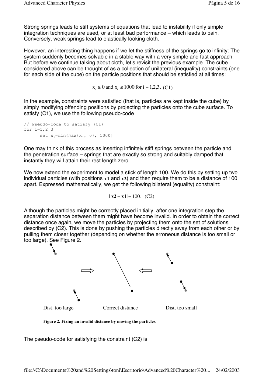(C2) = | 100 Although the particles might be correctly placed initially, after one integration step the separation distance between them might have become invalid. In order to obtain the correct distance once again, we move the particles by projecting them onto the set of solutions described by (C2). This is done by pushing the particles directly away from each other or by pulling them closer together (depending on whether the erroneous distance is too small or too large). See Figure 2. Dist. too large Correct distance Dist. too small Figure 2. Fixing an invalid distance by moving the particles. The pseudo-code for satisfying the constraint (C2) is file://C:\Documents%20and%20Settings\toni\Escritorio\Advanced%20Character%20... 24/02/2003

Advanced Character Physics Página 6 de 16 // Pseudo-code to satisfy (C2) delta = x2-x1; deltalength = sqrt(delta*delta); diff = (deltalength-restlength)/deltalength; x1 += delta*0.5*diff; x2 -= delta*0.5*diff; Note that delta is a vector so delta*delta is actually a dot product. With restlength=100 the above pseudo-code will push apart or pull together the particles such that they once more attain the correct distance of 100 between them. Again we may think of the situation as if a very stiff spring with rest length 100 has been inserted between the particles such that they are instantly placed correctly. Now assume that we still want the particles to satisfy the cube constraints. By satisfying the stick constraint, however, we may have invalidated one or more of the cube constraints by pushing a particle out of the cube. This situation can be remedied by immediately projecting the offending particle position back onto the cube surface once more – but then we end up invalidating the stick constraint again. Really, what we should do is solve for all constraints at once, both (C1) and (C2). This would be a matter of solving a system of equations. However, we choose to proceed indirectly by local iteration. We simply repeat the two pieces of pseudo-code a number of times after each other in the hope that the result is useful. This yields the following code: // Implements simulation of a stick in a box void ParticleSystem::SatisfyConstraints() { for(int j=0; j

Advanced Character Physics Página 7 de 16 This means that stopping early will not ruin everything although the resulting animation might appear somewhat sloppier. Cloth simulation The fact that a stick constraint can be thought of as a really hard spring should make apparent its usefulness for cloth simulation as sketched in the beginning of this section. Assume, for example, that a hexagonal mesh of triangles describing the cloth has been constructed. For each vertex a particle is initialized and for each edge a stick constraint between the two corresponding particles is initialized (with the constraint’s “rest length” simply being the initial distance between the two vertices). The function HandleConstraints() then uses relaxation over all constraints. The relaxation loop could be iterated several times. However, to obtain nicely looking animation, actually for most pieces of cloth only one iteration is necessary! This means that the time usage in the cloth simulation depends mostly on the N square root operations and the N divisions performed (where N denotes the number of edges in the cloth mesh). As we shall see, a clever trick makes it possible to reduce this to N divisions per frame update – this is really fast and one might argue that it probably can’t get much faster. // Implements cloth simulation struct Constraint { int particleA, particleB; float restlength; }; // Assume that an array of constraints, m_constraints, exists void ParticleSystem::SatisfyConstraints() { for(int j=0; j

Advanced Character Physics Página 8 de 16 Notice that if the distance is already correct (that is, if |delta|=restlength), then one gets delta=(0,0,0) and no change is going to happen. Per constraint we now use zero square roots, one division only, and the squared value restlength*restlength can even be precalculated! The usage of time consuming operations is now down to N divisions per frame (and the corresponding memory accesses) – it can’t be done much faster than that and the result even looks quite nice. Actually, in Hitman, the overall speed of the cloth simulation was limited mostly by how many triangles it was possible to push through the rendering system. The constraints are not guaranteed to be satisfied after one iteration only, but because of the Verlet integration scheme, the system will quickly converge to the correct state over some frames. In fact, using only one iteration and approximating the square root removes the stiffness that appears otherwise when the sticks are perfectly stiff. By placing support sticks between strategically chosen couples of vertices sharing a neighbor, the cloth algorithm can be extended to simulate plants. Again, in Hitman only one pass through the relaxation loop was enough (in fact, the low number gave the plants exactly the right amount of bending behavior). The code and the equations covered in this section assume that all particles have identical mass. Of course, it is possible to model particles with different masses, the equations only get a little more complex. To satisfy (C2) while respecting particle masses, use the following code: // Pseudo-code to satisfy (C2) delta = x2-x1; deltalength = sqrt(delta*delta); diff = (deltalength-restlength) x1 += invmass1*delta*diff; x2 -= invmass2*delta*diff; Here invmass1 and invmass2 are the numerical inverses of the two masses. If we want a particle to be immovable, simply set invmass=0 for that particle (corresponding to an infinite mass). Of course in the above case, the square root can also be approximated for a speed- up. 5 Rigid bodies The equations governing motion of rigid bodies were discovered long before the invention of modern computers. To be able to say anything useful at that time, mathematicians needed the ability to manipulate expressions symbolically. In the theory of rigid bodies, this lead to useful notions and tools such as inertia tensors, angular momentum, torque, quaternions for representing orientations etc. However, with the current ability to process huge amounts of data numerically, it has become feasible and in some cases even advantageous to break down calculations to simpler elements when running a simulation. In the case of 3D rigid bodies, this could mean modeling a rigid body by four particles and six constraints (giving the correct amount of degrees of freedom, 4x3-6 = 6). This simplifies a lot of aspects and it’s exactly what we will do in the following. Consider a tetrahedron and place a particle at each of the four vertices. In addition, for each of the six edges on the tetrahedron create a distance constraint like the stick constraint discussed in the previous section. This is actually enough to simulate a rigid body. The tetrahedron can be let loose inside the cube world from earlier and the Verlet integrator will let it move correctly. The function SatisfyConstraints() should take care of two /(deltalength*(invmass1+invmass2)); file://C:\Documents%20and%20Settings\toni\Escritorio\Advanced%20Character%20... 24/02/2003

分享到：

赞收藏

资料库

AdvancedCharacterPhysics.pdf

相关推荐

开发技术

热门标签

最新资料