Laplacian Score for Feature Selection
Xiaofei He1
Deng Cai2
Partha Niyogi1
1 Department of Computer Science, University of Chicago
{xiaofei, niyogi}@cs.uchicago.edu
2 Department of Computer Science, University of Illinois at Urbana-Champaign
dengcai2@uiuc.edu
Abstract
In supervised learning scenarios, feature selection has been studied
widely in the literature. Selecting features in unsupervised learning sce-
narios is a much harder problem, due to the absence of class labels that
would guide the search for relevant information. And, almost all of pre-
vious unsupervised feature selection methods are “wrapper” techniques
that require a learning algorithm to evaluate the candidate feature subsets.
In this paper, we propose a “filter” method for feature selection which is
independent of any learning algorithm. Our method can be performed in
either supervised or unsupervised fashion. The proposed method is based
on the observation that, in many real world classification problems, data
from the same class are often close to each other. The importance of a
feature is evaluated by its power of locality preserving, or, Laplacian
Score. We compare our method with data variance (unsupervised) and
Fisher score (supervised) on two data sets. Experimental results demon-
strate the effectiveness and efficiency of our algorithm.
1
Introduction
Feature selection methods can be classified into “wrapper” methods and “filter” methods
[4]. The wrapper model techniques evaluate the features using the learning algorithm that
will ultimately be employed. Thus, they “wrap” the selection process around the learning
algorithm. Most of the feature selection methods are wrapper methods. Algorithms based
on the filter model examine intrinsic properties of the data to evaluate the features prior to
the learning tasks. The filter based approaches almost always rely on the class labels, most
commonly assessing correlations between features and the class label. In this paper, we
are particularly interested in the filter methods. Some typical filter methods include data
variance, Pearson correlation coefficients, Fisher score, and Kolmogorov-Smirnov test.
Most of the existing filter methods are supervised. Data variance might be the simplest
unsupervised evaluation of the features. The variance along a dimension reflects its repre-
sentative power. Data variance can be used as a criteria for feature selection and extraction.
For example, Principal Component Analysis (PCA) is a classical feature extraction method
which finds a set of mutually orthogonal basis functions that capture the directions of max-
imum variance in the data.
Although the data variance criteria finds features that are useful for representing data, there
�
is no reason to assume that these features must be useful for discriminating between data in
different classes. Fisher score seeks features that are efficient for discrimination. It assigns
the highest score to the feature on which the data points of different classes are far from
each other while requiring data points of the same class to be close to each other. Fisher
criterion can be also used for feature extraction, such as Linear Discriminant Analysis
(LDA).
In this paper, we introduce a novel feature selection algorithm called Laplacian Score (LS).
For each feature, its Laplacian score is computed to reflect its locality preserving power.
LS is based on the observation that, two data points are probably related to the same topic
if they are close to each other. In fact, in many learning problems such as classification,
the local structure of the data space is more important than the global structure. In order to
model the local geometric structure, we construct a nearest neighbor graph. LS seeks those
features that respect this graph structure.
2 Laplacian Score
Laplacian Score (LS) is fundamentally based on Laplacian Eigenmaps [1] and Locality
Preserving Projection [3]. The basic idea of LS is to evaluate the features according to their
locality preserving power.
2.1 The Algorithm
Let Lr denote the Laplacian Score of the r-th feature. Let fri denote the i-th sample of the
r-th feature, i = 1, · · · , m. Our algorithm can be stated as follows:
1. Construct a nearest neighbor graph G with m nodes. The i-th node corresponds
to xi. We put an edge between nodes i and j if xi and xj are ”close”, i.e. xi is
among k nearest neighbors of xj or xj is among k nearest neighbors of xi. When
the label information is available, one can put an edge between two nodes sharing
the same label.
2. If nodes i and j are connected, put Sij = e−
, where t is a suitable constant.
Otherwise, put Sij = 0. The weight matrix S of the graph models the local
structure of the data space.
t
kxi−xj k2
3. For the r-th feature, we define:
fr = [fr1, fr2, · · · , frm]T , D = diag(S1), 1 = [1, · · · , 1]T , L = D − S
where the matrix L is often called graph Laplacian [2]. Let
4. Compute the Laplacian Score of the r-th feature as follows:
(1)
r D1
fT
1T D1
1
efr = fr −
Lr = efT
r Lefr
efT
r Defr
3
Justification
3.1 Objective Function
Recall that given a data set we construct a weighted graph G with edges connecting nearby
points to each other. Sij evaluates the similarity between the i-th and j-th nodes. Thus,
�
the importance of a feature can be thought of as the degree it respects the graph structure.
To be specific, a ”good” feature should the one on which two data points are close to each
other if and only if there is an edge between these two points. A reasonable criterion for
choosing a good feature is to minimize the following object function:
Lr = Pij(fri − frj)2Sij
V ar(fr)
(2)
where V ar(fr) is the estimated variance of the r-th feature. By minimizing Pij(fri −
frj)2Sij, we prefer those features respecting the pre-defined graph structure. For a good
feature, the bigger Sij, the smaller (fri − frj), and thus the Laplacian Score tends to be
small. Following some simple algebraic steps, we see that
Xij
= 2Xij
(fri − frj)2 Sij =Xij f 2
riSij − 2Xij
f 2
ri + f 2
rj − 2frifrj Sij
friSijfrj = 2fT
r Dfr − 2fT
r Sfr = 2fT
r Lfr
By maximizing V ar(fr), we prefer those features with large variance which have more
representative power. Recall that the variance of a random variable a can be written as
follows:
V ar(a) =ZM
(a − µ)2dP (a), µ =ZM
adP (a)
where M is the data manifold, µ is the expected value of a and dP is the probability
measure. By spectral graph theory [2], dP can be estimated by the diagonal matrix D on
the sample points. Thus, the weighted data variance can be estimated as follows:
µr =Pifri
V ar(fr) =Pi(fri − µr)2Dii
DiiP i Dii =
(Pi friDii) =
1
(P i Dii)
To remove the mean from the samples, we define:
fT
r D1
1T D1
Thus,
fT
r D1
1T D1
1
riDii =efT
r Defr
efr = fr −
V ar(fr) =Xi ef2
r Lefr = fT
r Lfr (please see Proposition 1 in Section 4.2 for
Also, it is easy to show thatefT
detials). We finally get equation (1).
It would be important to note that, if we do not remove the mean, the vector fr can be a non-
zero constant vector such as 1. It is easy to check that, 1T L1 = 0 and 1T D1 > 0. Thus,
Lr = 0. Unfortunately, this feature is clearly of no use since it contains no information.
With mean being removed, the new vectorefr is orthogonal to 1 with respect to D, i.e.
efT
r D1 = 0. Therefore,efr can not be any constant vector other than 0. Ifefr = 0,efT
r Lefr =
efT
r Defr = 0. Thus, the Laplacian Score Lr becomes a trivial solution and the r-th feature
is excluded from selection. While computing the weighted variance, the matrix D models
the importance (or local density) of the data points. We can also simply replace it by the
identity matrix I, in which case the weighted variance becomes the standard variance. To
be specific,
r I1
fT
1T I1
1 = fr −
r 1
fT
n
1 = fr − µ1
efr = fr −
�
where µ is the mean of fri, i = 1, · · · , n. Thus,
which is just the standard variance.
V ar(fr) =efT
r Iefr =
1
n
(fr − µ1)T (fr − µ1)
(3)
In fact, the Laplacian scores can be thought of as the Rayleigh quotients for the features
with respect to the graph G, please see [2] for details.
3.2 Connection to Fisher Score
In this section, we provide a theoretical analysis of the connection between our algorithm
and the canonical Fisher score.
Given a set of data points with label, {xi, yi}n
i=1, yi ∈ {1, · · · , c}. Let ni denote the
number of data points in class i. Let µi and σ2
i be the mean and variance of class i,
i = 1, · · · , c, corresponding to the r-th feature. Let µ and σ2 denote the mean and variance
of the whole data set. The Fisher score is defined below:
i=1 ni(µi − µ)2
(4)
Fr = Pc
i=1 niσ2
i
Pc
In the following, we show that Fisher score is equivalent to Laplacian score with a special
graph structure. We define the weight matrix as follows:
Sij = 1
nl
0,
,
yi = yj = l;
otherwise.
(5)
Without loss of generality, we assume that the data points are ordered according to which
class they are in, so that {x1, · · · , xn1} are in the first class, {xn1+1, · · · , xn1+n2} are in
the second class, etc. Thus, S can be written as follows:
S =
S1
0
0
0
...
0
0
0
Sc
where Si = 1
ni
to 1, so Di = diag(Si1) is just the identity matrix. Define f1
[fr,n1+1, · · · , fr,n1+n2]T , etc. We now make the following observations.
11T is an ni × ni matrix. For each Si, the raw (or column) sum is equal
r =
r = [fr1, · · · , frn1 ]T , f2
Observation 1 With the weight matrix S defined in (5), we haveefT
Pi niσ2
i , where L = D − S.
To see this, define Li = Di − Si = Ii − Si, where Ii is the ni × ni identity matrix. We
have
r Lefr = fT
r Lfr =
r Lfr =
fT
cXi=1
(fi
r)T Lifi
r =
cXi=1
(fi
r)T (Ii −
1
ni
11T )fi
r =
cXi=1
nicov(fi
r, fi
r) =
cXi=1
niσ2
i
Note that, since uT L1 = 1T Lu = 0, ∀u ∈ Rn, the value of fT
subtracting a constant vector (= α1) from fr. This shows thatefT
Observation 2 With the weight matrix S defined in (5), we haveefT
r Lefr = fT
r Defr = nσ2.
To see this, by the definition of S, we have D = I. Thus, this is a immediate result from
equation (3).
r Lfr remains unchanged by
i .
r Lfr =Pi niσ2
�
ni(µi − µ)2 =
To see this, notice
Observation 3 With the weight matrix S defined in (5), we have Pc
r Defr −efT
efT
r Lefr.
cXi=1
cXi=1
cXi=1
i − 2niµiµ + niµ2
cXi=1
cXi=1niµ2
cXi=1
ni (fi
(niµi)2 − 2µ
r Sfr − fT
r (
(nµ)2 = fT
rSifi
fi
r −
niµi + µ2
ni =
cXi=1
1
n
=
=
11T )fr
1
ni
1
n
i=1 ni(µi − µ)2 =
1
r)T 11T fi
r − 2nµ2 + nµ2
= fT
r (I − S)fr − fT
This completes the proof.
r (I −
1
n
11T )fr = fT
r −efT
r LefT
r Lfr − nσ2 =efT
r DefT
r
We therefore get the following relationship between the Laplacian score and Fisher score:
Theorem 1 Let Fr denote the Fisher score of the r-th feature. With the weight matrix S
defined in (5), we have Lr = 1
.
1+Fr
Proof From observations 1,2,3, we see that
Fr = Pc
i=1 ni(µi − µ)2
i=1 niσ2
i
Pc
Thus, Lr = 1
1+Fr
.
r
r LefT
r −efT
r DefT
=efT
r LefT
efT
r
=
1
Lr
− 1
4 Experimental Results
Several experiments were carried out to demonstrate the efficiency and effectiveness of our
algorithm. Our algorithm is a unsupervised filter method, while almost all the existing filter
methods are supervised. Therefore, we compared our algorithm with data variance which
can be performed in unsupervised fashion.
4.1 UCI Iris Data
Iris dataset, popularly used for testing clustering and classification algorithms, is taken from
UCI ML repository. It contains 3 classes of 50 instances each, where each class refers to
a type of Iris plant. Each instance is characterized by four features, i.e. sepal length, sepal
width, petal length, and petal width. One class is linearly separable from the other two,
but the other two are not linearly separable from each other. Out of the four features it is
known that the features F3 (petal length) and F4 (petal width) are more important for the
underlying clusters.
The class correlation for each feature is 0.7826, -0.4194, 0.9490 and 0.9565. We also used
leave-one-out strategy to do classification by using each single feature. We simply used the
nearest neighbor classifier. The classification error rates for the four features are 0.41, 0.52,
0.12 and 0.12, respectively. Our analysis indicates that F3 and F4 are better than F1 and F2
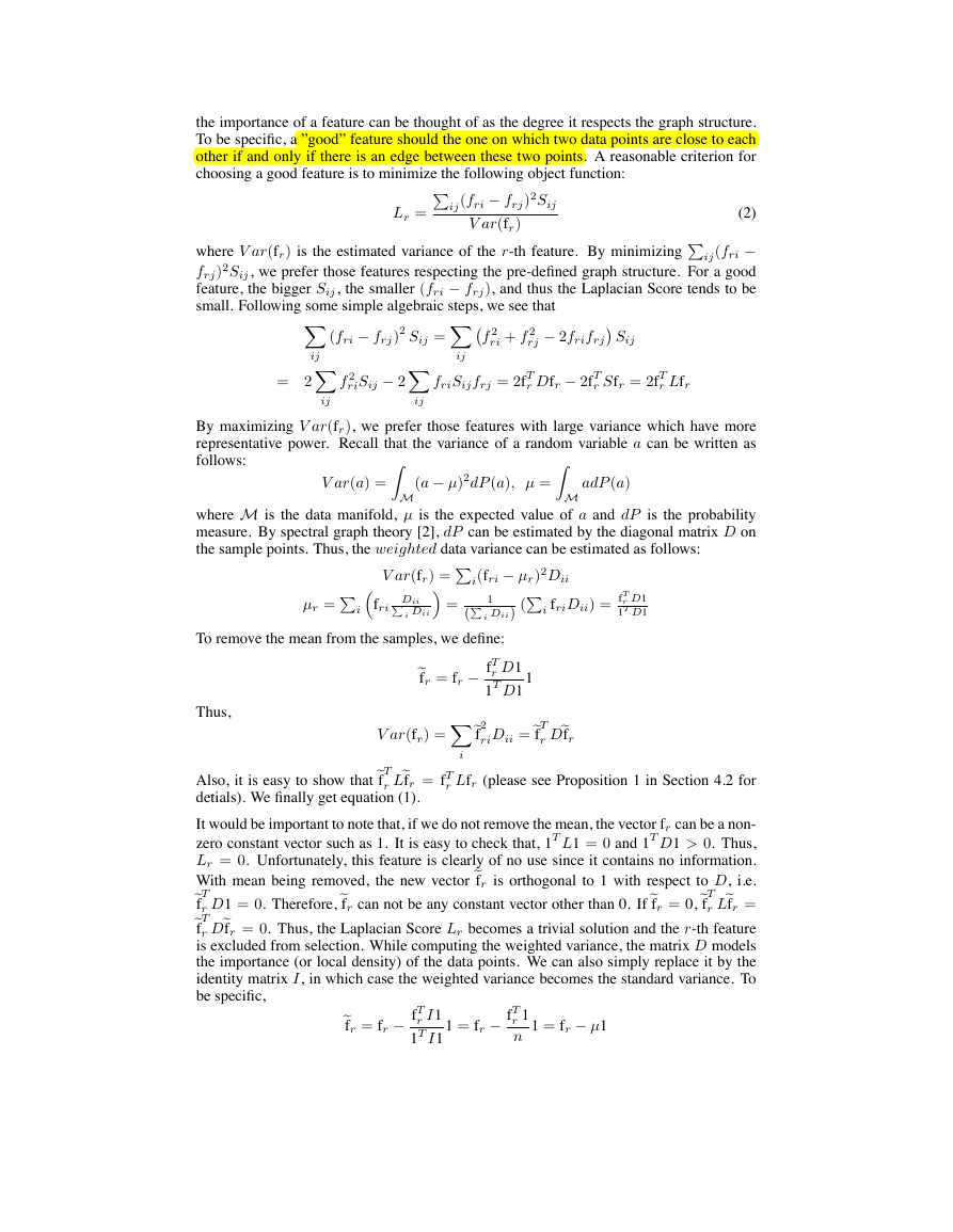
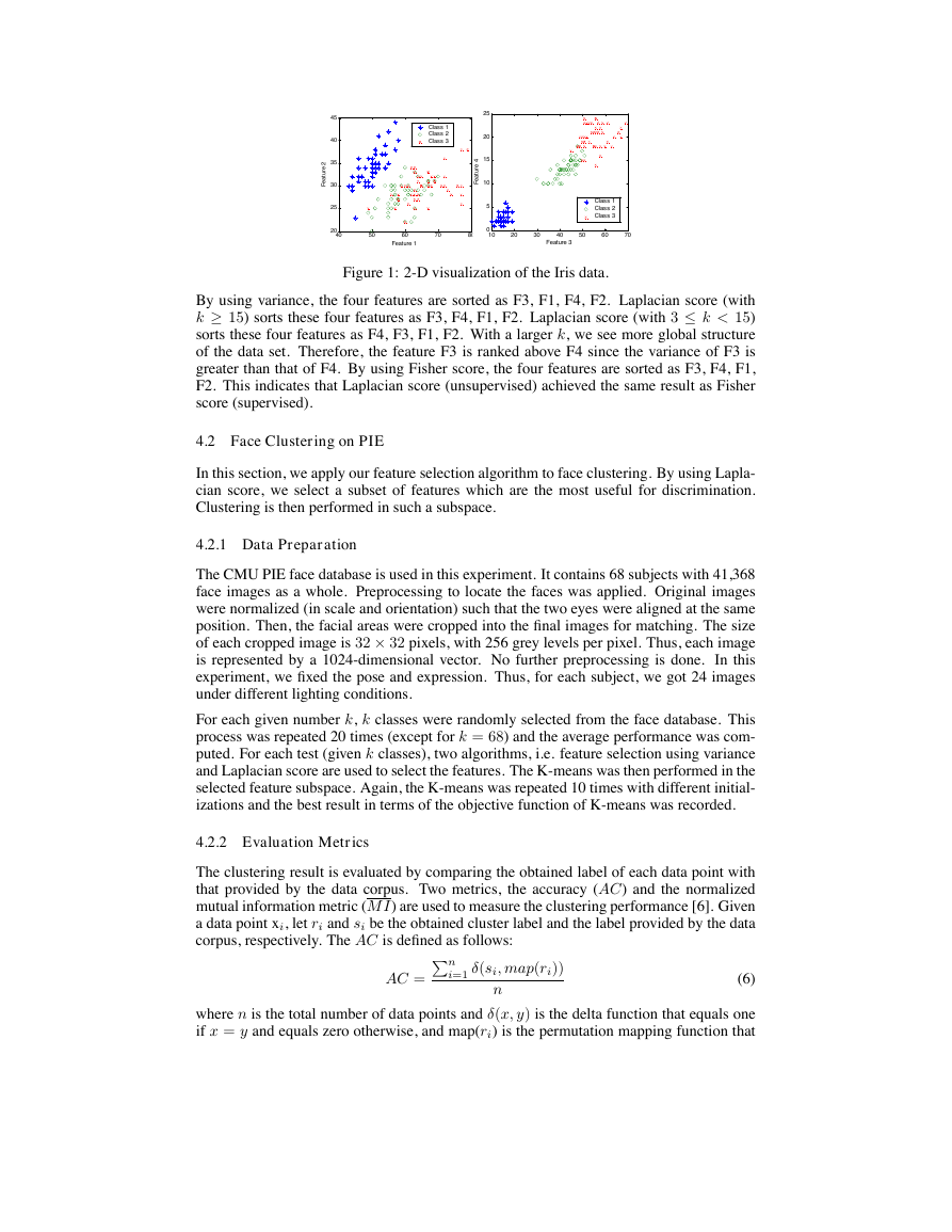
in the sense of discrimination. In figure 1, we present a 2-D visualization of the Iris data.
We compared three methods, i.e. Variance, Fisher score and Laplacian Score for feature
selection. All of them are filter methods which are independent to any learning tasks.
However, Fisher score is supervised, while the other two are unsupervised.
�
2
e
r
u
t
a
e
F
45
40
35
30
25
20
40
Class 1
Class 2
Class 3
50
60
Feature 1
70
25
20
15
10
5
4
e
r
u
t
a
e
F
0
10
80
Class 1
Class 2
Class 3
20
30
40
50
60
Feature 3
70
Figure 1: 2-D visualization of the Iris data.
By using variance, the four features are sorted as F3, F1, F4, F2. Laplacian score (with
k ≥ 15) sorts these four features as F3, F4, F1, F2. Laplacian score (with 3 ≤ k < 15)
sorts these four features as F4, F3, F1, F2. With a larger k, we see more global structure
of the data set. Therefore, the feature F3 is ranked above F4 since the variance of F3 is
greater than that of F4. By using Fisher score, the four features are sorted as F3, F4, F1,
F2. This indicates that Laplacian score (unsupervised) achieved the same result as Fisher
score (supervised).
4.2 Face Clustering on PIE
In this section, we apply our feature selection algorithm to face clustering. By using Lapla-
cian score, we select a subset of features which are the most useful for discrimination.
Clustering is then performed in such a subspace.
4.2.1 Data Preparation
The CMU PIE face database is used in this experiment. It contains 68 subjects with 41,368
face images as a whole. Preprocessing to locate the faces was applied. Original images
were normalized (in scale and orientation) such that the two eyes were aligned at the same
position. Then, the facial areas were cropped into the final images for matching. The size
of each cropped image is 32 × 32 pixels, with 256 grey levels per pixel. Thus, each image
is represented by a 1024-dimensional vector. No further preprocessing is done. In this
experiment, we fixed the pose and expression. Thus, for each subject, we got 24 images
under different lighting conditions.
For each given number k, k classes were randomly selected from the face database. This
process was repeated 20 times (except for k = 68) and the average performance was com-
puted. For each test (given k classes), two algorithms, i.e. feature selection using variance
and Laplacian score are used to select the features. The K-means was then performed in the
selected feature subspace. Again, the K-means was repeated 10 times with different initial-
izations and the best result in terms of the objective function of K-means was recorded.
4.2.2 Evaluation Metrics
The clustering result is evaluated by comparing the obtained label of each data point with
that provided by the data corpus. Two metrics, the accuracy (AC) and the normalized
mutual information metric (M I) are used to measure the clustering performance [6]. Given
a data point xi, let ri and si be the obtained cluster label and the label provided by the data
corpus, respectively. The AC is defined as follows:
AC = Pn
i=1 δ(si, map(ri))
n
(6)
where n is the total number of data points and δ(x, y) is the delta function that equals one
if x = y and equals zero otherwise, and map(ri) is the permutation mapping function that
�
y
c
a
r
u
c
c
A
0.9
0.8
0.7
0.6
0.5
0.4
0
y
c
a
r
u
c
c
A
0.7
0.65
0.6
0.55
0.5
0.45
0.4
0.35
0.3
0
Laplacian Score
Variance
0.9
0.8
0.7
0.6
0.5
n
o
i
t
a
m
r
o
f
n
I
l
a
u
t
u
M
Laplacian Score
Variance
y
c
a
r
u
c
c
A
0.8
0.7
0.6
0.5
0.4
Laplacian Score
Variance
Laplacian Score
Variance
0.9
0.85
0.8
0.75
0.7
0.65
0.6
0.55
n
o
i
t
a
m
r
o
n
f
I
l
t
a
u
u
M
200
400
600
800
1000
Number of features
0.4
0
200
400
600
800
1000
0
200
400
600
800
1000
Number of features
Number of features
0.5
0
200
400
600
800
1000
Number of features
(a) 5 classes
(b) 10 classes
Laplacian Score
Variance
n
o
i
t
a
m
r
o
n
f
I
l
t
a
u
u
M
Laplacian Score
Variance
0.85
0.8
0.75
0.7
0.65
0.6
200
400
600
800
1000
Number of features
0.55
0
200
400
600
800
1000
Number of features
(c) 30 classes
y
c
a
r
u
c
c
A
0.65
0.6
0.55
0.5
0.45
0.4
0.35
0.3
0.25
0
Laplacian Score
Variance
Laplacian Score
Variance
0.9
0.85
0.8
0.75
0.7
0.65
0.6
n
o
i
t
a
m
r
o
n
f
I
l
t
a
u
u
M
200
400
600
800
1000
Number of features
0.55
0
200
400
600
800
1000
Number of features
(d) 68 classes
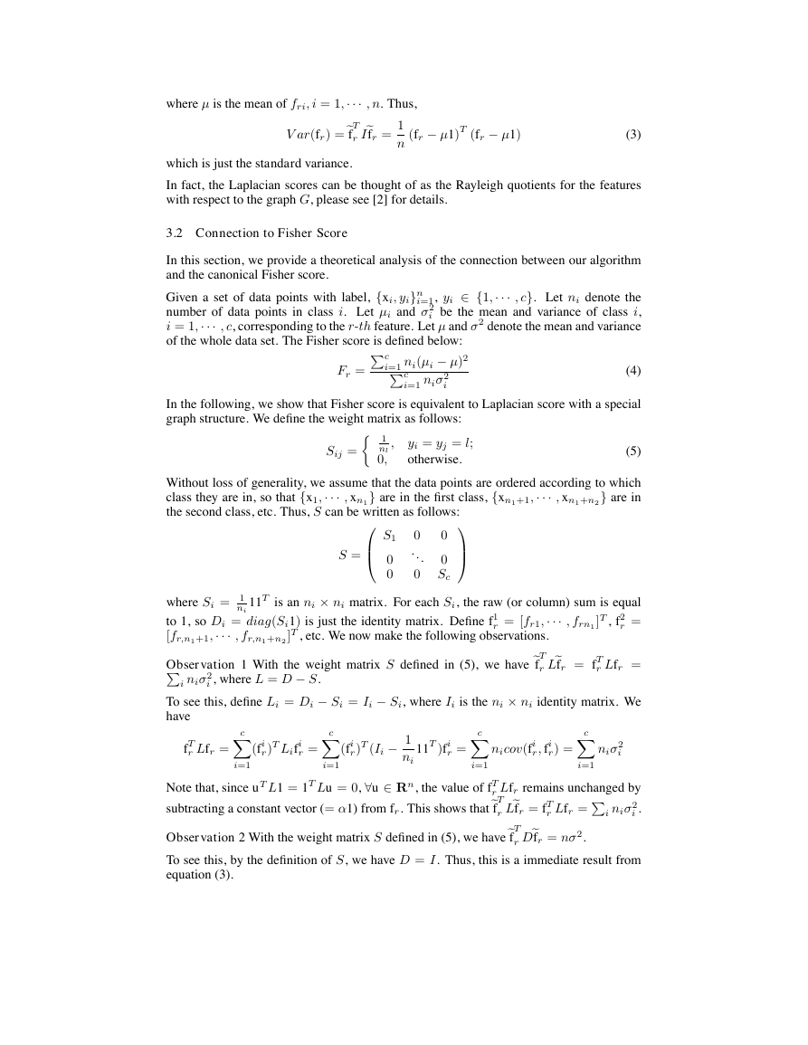
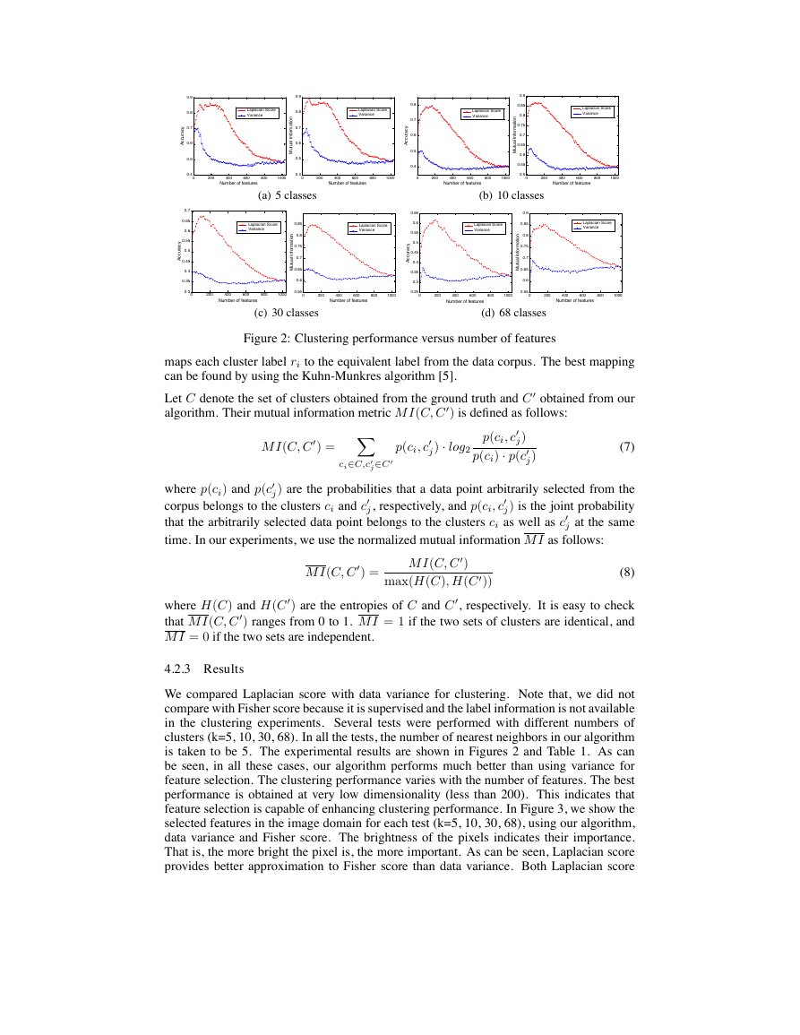
Figure 2: Clustering performance versus number of features
maps each cluster label ri to the equivalent label from the data corpus. The best mapping
can be found by using the Kuhn-Munkres algorithm [5].
Let C denote the set of clusters obtained from the ground truth and C 0 obtained from our
algorithm. Their mutual information metric M I(C, C 0) is defined as follows:
M I(C, C 0) = Xci∈C,c0
∈C0
j
p(ci, c0
j) · log2
p(ci, c0
j)
p(ci) · p(c0
j)
(7)
where p(ci) and p(c0
corpus belongs to the clusters ci and c0
that the arbitrarily selected data point belongs to the clusters ci as well as c0
time. In our experiments, we use the normalized mutual information M I as follows:
j) are the probabilities that a data point arbitrarily selected from the
j) is the joint probability
j at the same
j, respectively, and p(ci, c0
M I(C, C 0) =
M I(C, C 0)
max(H(C), H(C 0))
(8)
where H(C) and H(C 0) are the entropies of C and C 0, respectively. It is easy to check
that M I(C, C 0) ranges from 0 to 1. M I = 1 if the two sets of clusters are identical, and
M I = 0 if the two sets are independent.
4.2.3 Results
We compared Laplacian score with data variance for clustering. Note that, we did not
compare with Fisher score because it is supervised and the label information is not available
in the clustering experiments. Several tests were performed with different numbers of
clusters (k=5, 10, 30, 68). In all the tests, the number of nearest neighbors in our algorithm
is taken to be 5. The experimental results are shown in Figures 2 and Table 1. As can
be seen, in all these cases, our algorithm performs much better than using variance for
feature selection. The clustering performance varies with the number of features. The best
performance is obtained at very low dimensionality (less than 200). This indicates that
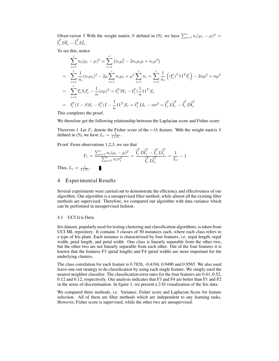
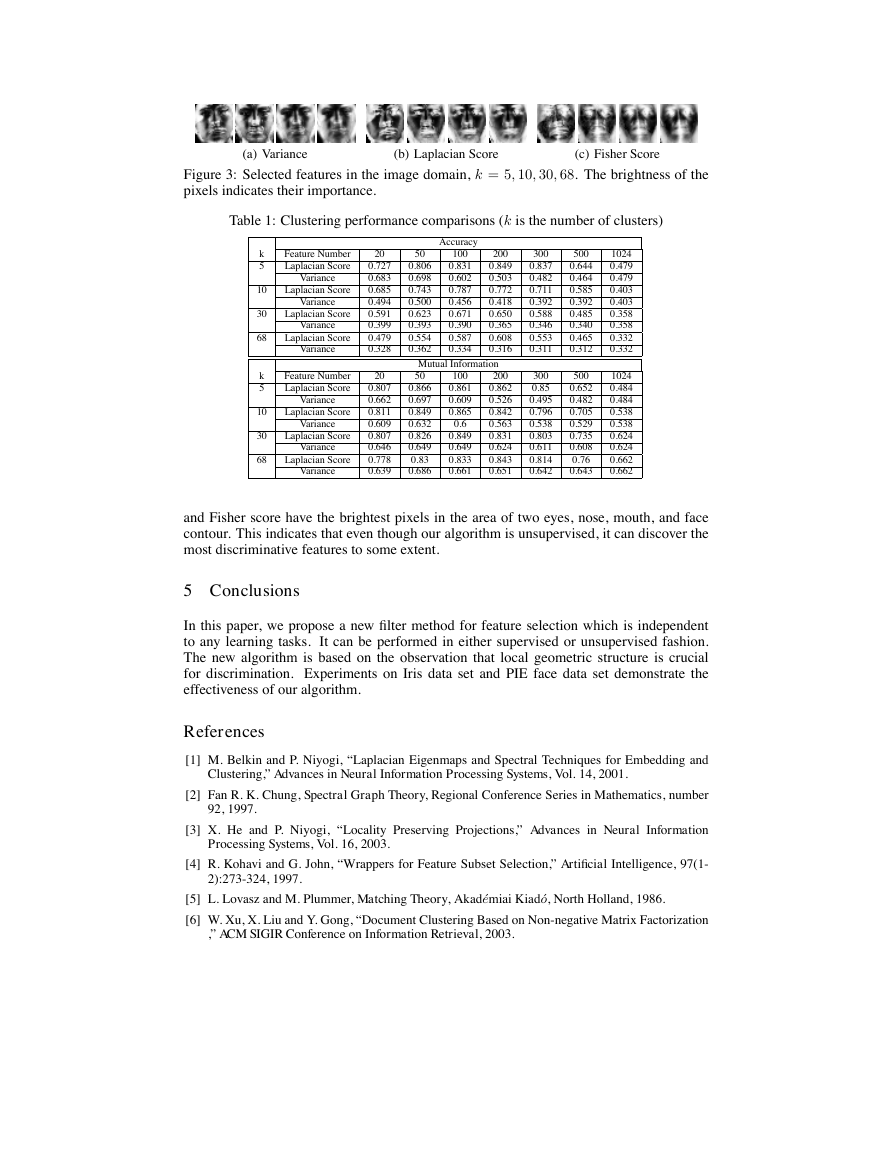
feature selection is capable of enhancing clustering performance. In Figure 3, we show the
selected features in the image domain for each test (k=5, 10, 30, 68), using our algorithm,
data variance and Fisher score. The brightness of the pixels indicates their importance.
That is, the more bright the pixel is, the more important. As can be seen, Laplacian score
provides better approximation to Fisher score than data variance. Both Laplacian score
�
(a) Variance
(b) Laplacian Score
(c) Fisher Score
Figure 3: Selected features in the image domain, k = 5, 10, 30, 68. The brightness of the
pixels indicates their importance.
Table 1: Clustering performance comparisons (k is the number of clusters)
k
5
10
30
68
k
5
10
30
68
Feature Number
Laplacian Score
Variance
Laplacian Score
Variance
Laplacian Score
Variance
Laplacian Score
Variance
Feature Number
Laplacian Score
Variance
Laplacian Score
Variance
Laplacian Score
Variance
Laplacian Score
Variance
20
0.727
0.683
0.685
0.494
0.591
0.399
0.479
0.328
20
0.807
0.662
0.811
0.609
0.807
0.646
0.778
0.639
0.866
0.697
0.849
0.632
0.826
0.649
0.83
0.686
Accuracy
100
0.831
0.602
0.787
0.456
0.671
0.390
0.587
0.334
50
0.806
0.698
0.743
0.500
0.623
0.393
0.554
0.362
200
0.849
0.503
0.772
0.418
0.650
0.365
0.608
0.316
Mutual Information
50
100
0.861
0.609
0.865
0.6
0.849
0.649
0.833
0.661
200
0.862
0.526
0.842
0.563
0.831
0.624
0.843
0.651
300
0.837
0.482
0.711
0.392
0.588
0.346
0.553
0.311
300
0.85
0.495
0.796
0.538
0.803
0.611
0.814
0.642
500
0.644
0.464
0.585
0.392
0.485
0.340
0.465
0.312
500
0.652
0.482
0.705
0.529
0.735
0.608
0.76
0.643
1024
0.479
0.479
0.403
0.403
0.358
0.358
0.332
0.332
1024
0.484
0.484
0.538
0.538
0.624
0.624
0.662
0.662
and Fisher score have the brightest pixels in the area of two eyes, nose, mouth, and face
contour. This indicates that even though our algorithm is unsupervised, it can discover the
most discriminative features to some extent.
5 Conclusions
In this paper, we propose a new filter method for feature selection which is independent
to any learning tasks. It can be performed in either supervised or unsupervised fashion.
The new algorithm is based on the observation that local geometric structure is crucial
for discrimination. Experiments on Iris data set and PIE face data set demonstrate the
effectiveness of our algorithm.
References
[1] M. Belkin and P. Niyogi, “Laplacian Eigenmaps and Spectral Techniques for Embedding and
Clustering,” Advances in Neural Information Processing Systems, Vol. 14, 2001.
[2] Fan R. K. Chung, Spectral Graph Theory, Regional Conference Series in Mathematics, number
92, 1997.
[3] X. He and P. Niyogi, “Locality Preserving Projections,” Advances in Neural Information
Processing Systems, Vol. 16, 2003.
[4] R. Kohavi and G. John, “Wrappers for Feature Subset Selection,” Artificial Intelligence, 97(1-
2):273-324, 1997.
[5] L. Lovasz and M. Plummer, Matching Theory, Akad´emiai Kiad´o, North Holland, 1986.
[6] W. Xu, X. Liu and Y. Gong, “Document Clustering Based on Non-negative Matrix Factorization
,” ACM SIGIR Conference on Information Retrieval, 2003.
�



 2023年江西萍乡中考道德与法治真题及答案.doc
 2012年重庆南川中考生物真题及答案.doc
 2013年江西师范大学地理学综合及文艺理论基础考研真题.doc
 2020年四川甘孜小升初语文真题及答案I卷.doc
 2020年注册岩土工程师专业基础考试真题及答案.doc
 2023-2024学年福建省厦门市九年级上学期数学月考试题及答案.doc
 2021-2022学年辽宁省沈阳市大东区九年级上学期语文期末试题及答案.doc
 2022-2023学年北京东城区初三第一学期物理期末试卷及答案.doc
 2018上半年江西教师资格初中地理学科知识与教学能力真题及答案.doc
 2012年河北国家公务员申论考试真题及答案-省级.doc
 2020-2021学年江苏省扬州市江都区邵樊片九年级上学期数学第一次质量检测试题及答案.doc
 2022下半年黑龙江教师资格证中学综合素质真题及答案.doc