7
1
0
2
n
u
J
5
]
L
C
.
s
c
[
1
v
7
2
4
1
0
.
6
0
7
1
:
v
i
X
r
a
A simple neural network module
for relational reasoning
Adam Santoro∗, David Raposo∗, David G.T. Barrett, Mateusz Malinowski,
Razvan Pascanu, Peter Battaglia, Timothy Lillicrap
adamsantoro@, draposo@, barrettdavid@, mateuszm@,
razp@, peterbattaglia@, countzero@google.com
DeepMind
London, United Kingdom
Abstract
Relational reasoning is a central component of generally intelligent behavior, but has proven
difficult for neural networks to learn. In this paper we describe how to use Relation Networks
(RNs) as a simple plug-and-play module to solve problems that fundamentally hinge on relational
reasoning. We tested RN-augmented networks on three tasks: visual question answering
using a challenging dataset called CLEVR, on which we achieve state-of-the-art, super-human
performance; text-based question answering using the bAbI suite of tasks; and complex reasoning
about dynamic physical systems. Then, using a curated dataset called Sort-of-CLEVR we show
that powerful convolutional networks do not have a general capacity to solve relational questions,
but can gain this capacity when augmented with RNs. Our work shows how a deep learning
architecture equipped with an RN module can implicitly discover and learn to reason about
entities and their relations.
1
Introduction
The ability to reason about the relations between entities and their properties is central to generally
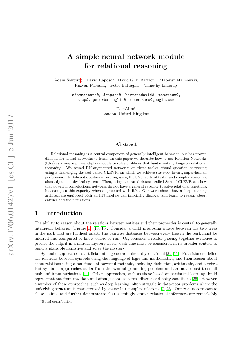
intelligent behavior (Figure 1) [18, 15]. Consider a child proposing a race between the two trees
in the park that are furthest apart: the pairwise distances between every tree in the park must be
inferred and compared to know where to run. Or, consider a reader piecing together evidence to
predict the culprit in a murder-mystery novel: each clue must be considered in its broader context to
build a plausible narrative and solve the mystery.
Symbolic approaches to artificial intelligence are inherently relational [32, 11]. Practitioners define
the relations between symbols using the language of logic and mathematics, and then reason about
these relations using a multitude of powerful methods, including deduction, arithmetic, and algebra.
But symbolic approaches suffer from the symbol grounding problem and are not robust to small
task and input variations [11]. Other approaches, such as those based on statistical learning, build
representations from raw data and often generalize across diverse and noisy conditions [25]. However,
a number of these approaches, such as deep learning, often struggle in data-poor problems where the
underlying structure is characterized by sparse but complex relations [7, 23]. Our results corroborate
these claims, and further demonstrate that seemingly simple relational inferences are remarkably
∗Equal contribution.
1
�
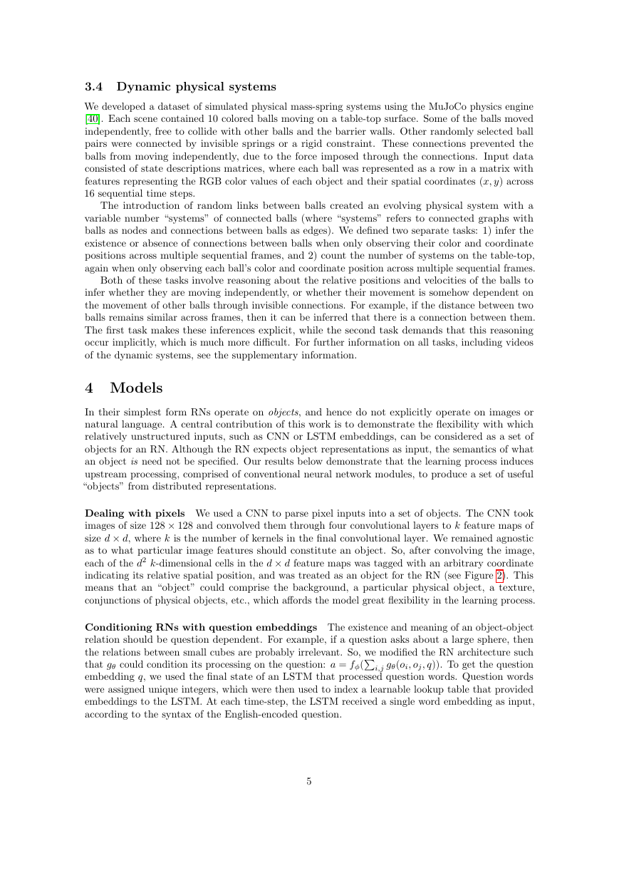
Figure 1: An illustrative example from the CLEVR dataset of relational reasoning. An
image containing four objects is shown alongside non-relational and relational questions. The
relational question requires explicit reasoning about the relations between the four objects in the
image, whereas the non-relational question requires reasoning about the attributes of a particular
object.
difficult for powerful neural network architectures such as convolutional neural networks (CNNs) and
multi-layer perceptrons (MLPs).
Here, we explore “Relation Networks” (RN) as a general solution to relational reasoning in neural
networks. RNs are architectures whose computations focus explicitly on relational reasoning [35].
Although several other models supporting relation-centric computation have been proposed, such
as Graph Neural Networks, Gated Graph Sequence Neural Networks, and Interaction Networks,
[37, 26, 2], RNs are simple, plug-and-play, and are exclusively focused on flexible relational reasoning.
Moreover, through joint training RNs can influence and shape upstream representations in CNNs
and LSTMs to produce implicit object-like representations that it can exploit for relational reasoning.
We applied an RN-augmented architecture to CLEVR [15], a recent visual question answering
(QA) dataset on which state-of-the-art approaches have struggled due to the demand for rich
relational reasoning. Our networks vastly outperformed the best generally-applicable visual QA
architectures, and achieve state-of-the-art, super-human performance. RNs also solve CLEVR from
state descriptions, highlighting their versatility in regards to the form of their input. We also applied
an RN-based architecture to the bAbI text-based QA suite [41] and solved 18/20 of the subtasks.
Finally, we trained an RN to make challenging relational inferences about complex physical systems
and motion capture data. The success of RNs across this set of substantially dissimilar task domains
is testament to the general utility of RNs for solving problems that require relation reasoning.
2 Relation Networks
An RN is a neural network module with a structure primed for relational reasoning. The design
philosophy behind RNs is to constrain the functional form of a neural network so that it captures the
core common properties of relational reasoning. In other words, the capacity to compute relations
is baked into the RN architecture without needing to be learned, just as the capacity to reason
about spatial, translation invariant properties is built-in to CNNs, and the capacity to reason about
sequential dependencies is built into recurrent neural networks.
In its simplest form the RN is a composite function:
,
RN(O) = fφ
gθ(oi, oj)
(1)
where the input is a set of “objects” O = {o1, o2, ..., on}, oi ∈ Rm is the ith object, and fφ and gθ
are functions with parameters φ and θ, respectively. For our purposes, fφ and gθ are MLPs, and the
i,j
2
What is the size of the brown sphere?Non-relational question:Original Image:Relational question:Are there any rubber things that have the same size as the yellow metallic cylinder?�
parameters are learnable synaptic weights, making RNs end-to-end differentiable. We call the output
of gθ a “relation”; therefore, the role of gθ is to infer the ways in which two objects are related, or if
they are even related at all.
RNs have three notable strengths: they learn to infer relations, they are data efficient, and they
operate on a set of objects – a particularly general and versatile input format – in a manner that is
order invariant.
RNs learn to infer relations The functional form in Equation 1 dictates that an RN should
consider the potential relations between all object pairs. This implies that an RN is not necessarily
privy to which object relations actually exist, nor to the actual meaning of any particular relation.
Thus, RNs must learn to infer the existence and implications of object relations.
In graph theory parlance, the input can be thought of as a complete and directed graph whose
nodes are objects and whose edges denote the object pairs whose relations should be considered.
Although we focus on this “all-to-all” version of the RN throughout this paper, this RN definition
can be adjusted to consider only some object pairs. Similar to Interaction Networks [2], to which
RNs are related, RNs can take as input a list of only those pairs that should be considered, if this
information is available. This information could be explicit in the input data, or could perhaps be
extracted by some upstream mechanism.
RNs are data efficient RNs use a single function gθ to compute each relation. This can be
thought of as a single function operating on a batch of object pairs, where each member of the
batch is a particular object-object pair from the same object set. This mode of operation encourages
greater generalization for computing relations, since gθ is encouraged not to over-fit to the features
of any particular object pair. Consider how an MLP would learn the same function. An MLP would
receive all objects from the object set simultaneously as its input. It must then learn and embed n2
(where n is the number of objects) identical functions within its weight parameters to account for all
possible object pairings. This quickly becomes intractable as the number of objects grows. Therefore,
the cost of learning a relation function n2 times using a single feedforward pass per sample, as in an
MLP, is replaced by the cost of n2 feedforward passes per object set (i.e., for each possible object
pair in the set) and learning a relation function just once, as in an RN.
RNs operate on a set of objects The summation in Equation 1 ensures that the RN is invariant
to the order of objects in the input. This invariance ensures that the RN’s input respects the property
that sets are order invariant, and it ensures that the output is order invariant. Ultimately, this
invariance ensures that the RN’s output contains information that is generally representative of the
relations that exist in the object set.
3 Tasks
We applied RN-augmented networks to a variety of tasks that hinge on relational reasoning. To
demonstrate the versatility of these networks we chose tasks from a number of different domains,
including visual QA, text-based QA, and dynamic physical systems.
3.1 CLEVR
In visual QA a model must learn to answer questions about an image (Figure 1). This is a challenging
problem domain because it requires high-level scene understanding [1, 29]. Architectures must perform
complex relational reasoning – spatial and otherwise – over the features in the visual inputs, language
inputs, and their conjunction. However, the majority of visual QA datasets require reasoning in the
absence of fully specified word vocabularies, and perhaps more perniciously, a vast and complicated
knowledge of the world that is not available in the training data. They also contain ambiguities and
exhibit strong linguistic biases that allow a model to learn answering strategies that exploit those
biases, without reasoning about the visual input [1, 31, 36].
3
�
To control for these issues, and to distill the core challenges of visual QA, the CLEVR visual QA
dataset was developed [15]. CLEVR contains images of 3D-rendered objects, such as spheres and
cylinders (Figure 2). Each image is associated with a number of questions that fall into different
categories. For example, query attribute questions may ask “What is the color of the sphere? ”,
while compare attribute questions may ask “Is the cube the same material as the cylinder? ”.
For our purposes, an important feature of CLEVR is that many questions are explicitly relational
in nature. Remarkably, powerful QA architectures [46] are unable to solve CLEVR, presumably
because they cannot handle core relational aspects of the task. For example, as reported in the
original paper a model comprised of ResNet-101 image embeddings with LSTM question processing
and augmented with stacked attention modules vastly outperformed other models at an overall
performance of 68.5% (compared to 52.3% for the next best, and 92.6% human performance) [15].
However, for compare attribute and count questions (i.e., questions heavily involving relations
across objects), the model performed little better than the simplest baseline, which answered questions
solely based on the probability of answers in the training set for a given question category (Q-type
baseline).
We used two versions of the CLEVR dataset: (i) the pixel version, in which images were
represented in standard 2D pixel form, and (ii) a state description version, in which images were
explicitly represented by state description matrices containing factored object descriptions. Each
row in the matrix contained the features of a single object – 3D coordinates (x, y, z); color (r, g,
b); shape (cube, cylinder, etc.); material (rubber, metal, etc.); size (small, large, etc.). When we
trained our models, we used either the pixel version or the state description version, depending on
the experiment, but not both together.
3.2 Sort-of-CLEVR
To explore our hypothesis that the RN architecture is better suited to general relational reasoning as
compared to more standard neural architectures, we constructed a dataset similar to CLEVR that
we call “Sort-of-CLEVR”1. This dataset separates relational and non-relational questions.
Sort-of-CLEVR consists of images of 2D colored shapes along with questions and answers about
the images. Each image has a total of 6 objects, where each object is a randomly chosen shape
(square or circle). We used 6 colors (red, blue, green, orange, yellow, gray) to unambiguously identify
each object. Questions are hard-coded as fixed-length binary strings to reduce the difficulty involved
with natural language question-word processing, and thereby remove any confounding difficulty
with language parsing. For each image we generated 10 relational questions and 10 non-relational
questions. Examples of relational questions are: “What is the shape of the object that is farthest from
the gray object? ”; and “How many objects have the same shape as the green object? ”. Examples of
non-relational questions are: “What is the shape of the gray object?”; and “Is the blue object on the
top or bottom of the scene? ”. The dataset is also visually simple, reducing complexities involved in
image processing.
3.3 bAbI
bAbI is a pure text-based QA dataset [41]. There are 20 tasks, each corresponding to a particular
type of reasoning, such as deduction, induction, or counting. Each question is associated with a set
of supporting facts. For example, the facts “Sandra picked up the football ” and “Sandra went to
the office” support the question “Where is the football? ” (answer: “office”). A model succeeds on
a task if its performance surpasses 95%. Many memory-augmented neural networks have reported
impressive results on bAbI. When training jointly on all tasks using 10K examples per task, Memory
Networks pass 14/20, DNC 18/20, Sparse DNC 19/20, and EntNet 16/20 (the authors of EntNets
report state-of-the-art at 20/20; however, unlike previously reported results this was not done with
joint training on all tasks, where they instead achieve 16/20) [42, 9, 34, 13].
1The “Sort-of-CLEVR” dataset will be made publicly available online.
4
�
3.4 Dynamic physical systems
We developed a dataset of simulated physical mass-spring systems using the MuJoCo physics engine
[40]. Each scene contained 10 colored balls moving on a table-top surface. Some of the balls moved
independently, free to collide with other balls and the barrier walls. Other randomly selected ball
pairs were connected by invisible springs or a rigid constraint. These connections prevented the
balls from moving independently, due to the force imposed through the connections. Input data
consisted of state descriptions matrices, where each ball was represented as a row in a matrix with
features representing the RGB color values of each object and their spatial coordinates (x, y) across
16 sequential time steps.
The introduction of random links between balls created an evolving physical system with a
variable number “systems” of connected balls (where “systems” refers to connected graphs with
balls as nodes and connections between balls as edges). We defined two separate tasks: 1) infer the
existence or absence of connections between balls when only observing their color and coordinate
positions across multiple sequential frames, and 2) count the number of systems on the table-top,
again when only observing each ball’s color and coordinate position across multiple sequential frames.
Both of these tasks involve reasoning about the relative positions and velocities of the balls to
infer whether they are moving independently, or whether their movement is somehow dependent on
the movement of other balls through invisible connections. For example, if the distance between two
balls remains similar across frames, then it can be inferred that there is a connection between them.
The first task makes these inferences explicit, while the second task demands that this reasoning
occur implicitly, which is much more difficult. For further information on all tasks, including videos
of the dynamic systems, see the supplementary information.
4 Models
In their simplest form RNs operate on objects, and hence do not explicitly operate on images or
natural language. A central contribution of this work is to demonstrate the flexibility with which
relatively unstructured inputs, such as CNN or LSTM embeddings, can be considered as a set of
objects for an RN. Although the RN expects object representations as input, the semantics of what
an object is need not be specified. Our results below demonstrate that the learning process induces
upstream processing, comprised of conventional neural network modules, to produce a set of useful
“objects” from distributed representations.
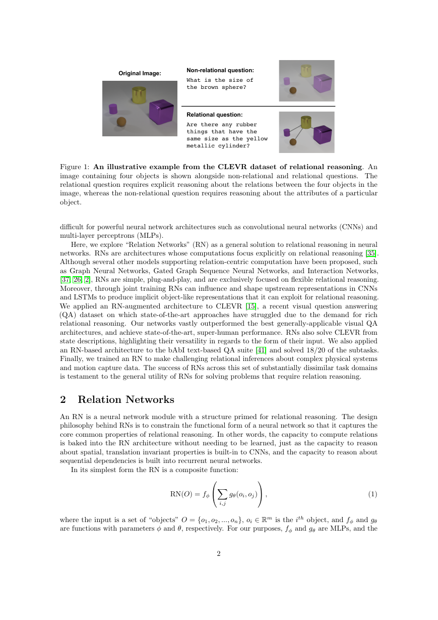
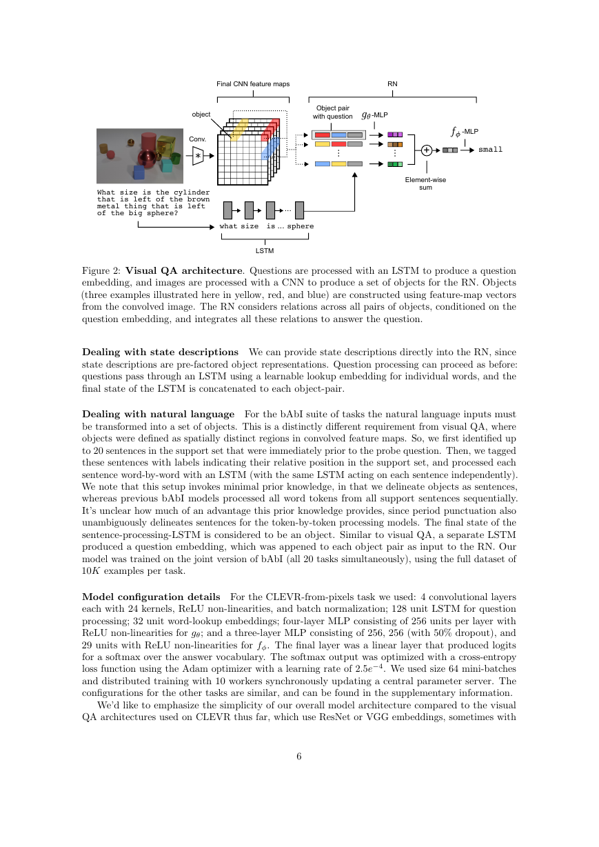
Dealing with pixels We used a CNN to parse pixel inputs into a set of objects. The CNN took
images of size 128 × 128 and convolved them through four convolutional layers to k feature maps of
size d × d, where k is the number of kernels in the final convolutional layer. We remained agnostic
as to what particular image features should constitute an object. So, after convolving the image,
each of the d2 k-dimensional cells in the d × d feature maps was tagged with an arbitrary coordinate
indicating its relative spatial position, and was treated as an object for the RN (see Figure 2). This
means that an “object” could comprise the background, a particular physical object, a texture,
conjunctions of physical objects, etc., which affords the model great flexibility in the learning process.
that gθ could condition its processing on the question: a = fφ(
Conditioning RNs with question embeddings The existence and meaning of an object-object
relation should be question dependent. For example, if a question asks about a large sphere, then
the relations between small cubes are probably irrelevant. So, we modified the RN architecture such
i,j gθ(oi, oj, q)). To get the question
embedding q, we used the final state of an LSTM that processed question words. Question words
were assigned unique integers, which were then used to index a learnable lookup table that provided
embeddings to the LSTM. At each time-step, the LSTM received a single word embedding as input,
according to the syntax of the English-encoded question.
5
�
Figure 2: Visual QA architecture. Questions are processed with an LSTM to produce a question
embedding, and images are processed with a CNN to produce a set of objects for the RN. Objects
(three examples illustrated here in yellow, red, and blue) are constructed using feature-map vectors
from the convolved image. The RN considers relations across all pairs of objects, conditioned on the
question embedding, and integrates all these relations to answer the question.
Dealing with state descriptions We can provide state descriptions directly into the RN, since
state descriptions are pre-factored object representations. Question processing can proceed as before:
questions pass through an LSTM using a learnable lookup embedding for individual words, and the
final state of the LSTM is concatenated to each object-pair.
Dealing with natural language For the bAbI suite of tasks the natural language inputs must
be transformed into a set of objects. This is a distinctly different requirement from visual QA, where
objects were defined as spatially distinct regions in convolved feature maps. So, we first identified up
to 20 sentences in the support set that were immediately prior to the probe question. Then, we tagged
these sentences with labels indicating their relative position in the support set, and processed each
sentence word-by-word with an LSTM (with the same LSTM acting on each sentence independently).
We note that this setup invokes minimal prior knowledge, in that we delineate objects as sentences,
whereas previous bAbI models processed all word tokens from all support sentences sequentially.
It’s unclear how much of an advantage this prior knowledge provides, since period punctuation also
unambiguously delineates sentences for the token-by-token processing models. The final state of the
sentence-processing-LSTM is considered to be an object. Similar to visual QA, a separate LSTM
produced a question embedding, which was appened to each object pair as input to the RN. Our
model was trained on the joint version of bAbI (all 20 tasks simultaneously), using the full dataset of
10K examples per task.
Model configuration details For the CLEVR-from-pixels task we used: 4 convolutional layers
each with 24 kernels, ReLU non-linearities, and batch normalization; 128 unit LSTM for question
processing; 32 unit word-lookup embeddings; four-layer MLP consisting of 256 units per layer with
ReLU non-linearities for gθ; and a three-layer MLP consisting of 256, 256 (with 50% dropout), and
29 units with ReLU non-linearities for fφ. The final layer was a linear layer that produced logits
for a softmax over the answer vocabulary. The softmax output was optimized with a cross-entropy
loss function using the Adam optimizer with a learning rate of 2.5e−4. We used size 64 mini-batches
and distributed training with 10 workers synchronously updating a central parameter server. The
configurations for the other tasks are similar, and can be found in the supplementary information.
We’d like to emphasize the simplicity of our overall model architecture compared to the visual
QA architectures used on CLEVR thus far, which use ResNet or VGG embeddings, sometimes with
6
small+-MLP............isspherewhatsizeFinal CNN feature mapsRNLSTMobject-MLPConv.What size is the cylinder that is left of the brown metal thing that is left of the big sphere?*Object pair with questionElement-wise sum�
Overall
Count
Exist
Compare
Numbers
Query
Attribute
Compare
Attribute
92.6
41.8
46.8
52.3
68.5
76.6
86.7
34.6
41.7
43.7
52.2
64.4
96.6
50.2
61.1
65.2
71.1
82.7
86.5
51.0
69.8
67.1
73.5
77.4
95.0
36.0
36.8
49.3
85.3
82.6
97.9
96.0
51.3
51.8
53.0
52.3
75.4
97.1
Model
Human
Q-type baseline
LSTM
CNN+LSTM
CNN+LSTM+SA
CNN+LSTM+SA*
CNN+LSTM+RN
95.5
90.1
97.8
93.6
* Our implementation, with optimized hyperparameters and trained fully end-to-end.
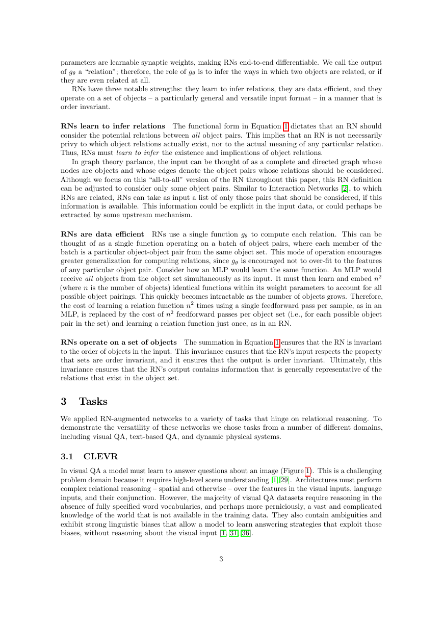
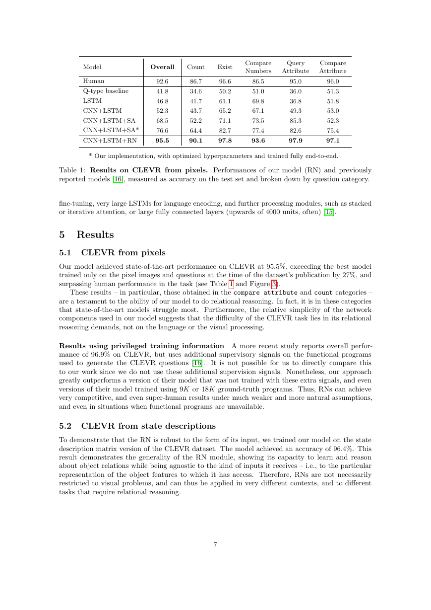
Table 1: Results on CLEVR from pixels. Performances of our model (RN) and previously
reported models [16], measured as accuracy on the test set and broken down by question category.
fine-tuning, very large LSTMs for language encoding, and further processing modules, such as stacked
or iterative attention, or large fully connected layers (upwards of 4000 units, often) [15].
5 Results
5.1 CLEVR from pixels
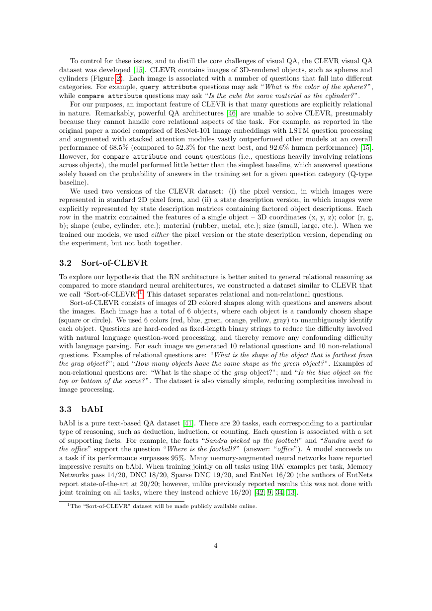
Our model achieved state-of-the-art performance on CLEVR at 95.5%, exceeding the best model
trained only on the pixel images and questions at the time of the dataset’s publication by 27%, and
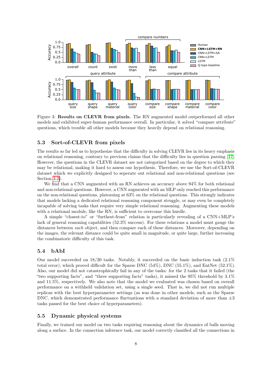
surpassing human performance in the task (see Table 1 and Figure 3).
These results – in particular, those obtained in the compare attribute and count categories –
are a testament to the ability of our model to do relational reasoning. In fact, it is in these categories
that state-of-the-art models struggle most. Furthermore, the relative simplicity of the network
components used in our model suggests that the difficulty of the CLEVR task lies in its relational
reasoning demands, not on the language or the visual processing.
Results using privileged training information A more recent study reports overall perfor-
mance of 96.9% on CLEVR, but uses additional supervisory signals on the functional programs
used to generate the CLEVR questions [16].
It is not possible for us to directly compare this
to our work since we do not use these additional supervision signals. Nonetheless, our approach
greatly outperforms a version of their model that was not trained with these extra signals, and even
versions of their model trained using 9K or 18K ground-truth programs. Thus, RNs can achieve
very competitive, and even super-human results under much weaker and more natural assumptions,
and even in situations when functional programs are unavailable.
5.2 CLEVR from state descriptions
To demonstrate that the RN is robust to the form of its input, we trained our model on the state
description matrix version of the CLEVR dataset. The model achieved an accuracy of 96.4%. This
result demonstrates the generality of the RN module, showing its capacity to learn and reason
about object relations while being agnostic to the kind of inputs it receives – i.e., to the particular
representation of the object features to which it has access. Therefore, RNs are not necessarily
restricted to visual problems, and can thus be applied in very different contexts, and to different
tasks that require relational reasoning.
7
�
Figure 3: Results on CLEVR from pixels. The RN augmented model outperformed all other
models and exhibited super-human performance overall. In particular, it solved “compare attribute”
questions, which trouble all other models because they heavily depend on relational reasoning.
5.3 Sort-of-CLEVR from pixels
The results so far led us to hypothesize that the difficulty in solving CLEVR lies in its heavy emphasis
on relational reasoning, contrary to previous claims that the difficulty lies in question parsing [17].
However, the questions in the CLEVR dataset are not categorized based on the degree to which they
may be relational, making it hard to assess our hypothesis. Therefore, we use the Sort-of-CLEVR
dataset which we explicitly designed to seperate out relational and non-relational questions (see
Section 3.2).
We find that a CNN augmented with an RN achieves an accuracy above 94% for both relational
and non-relational questions. However, a CNN augmented with an MLP only reached this performance
on the non-relational questions, plateauing at 63% on the relational questions. This strongly indicates
that models lacking a dedicated relational reasoning component struggle, or may even be completely
incapable of solving tasks that require very simple relational reasoning. Augmenting these models
with a relational module, like the RN, is sufficient to overcome this hurdle.
A simple “closest-to” or “furthest-from” relation is particularly revealing of a CNN+MLP’s
lack of general reasoning capabilities (52.3% success). For these relations a model must gauge the
distances between each object, and then compare each of these distances. Moreover, depending on
the images, the relevant distance could be quite small in magnitude, or quite large, further increasing
the combinatoric difficulty of this task.
5.4 bAbI
Our model succeeded on 18/20 tasks. Notably, it succeeded on the basic induction task (2.1%
total error), which proved difficult for the Sparse DNC (54%), DNC (55.1%), and EntNet (52.1%).
Also, our model did not catastrophically fail in any of the tasks: for the 2 tasks that it failed (the
“two supporting facts”, and “three supporting facts” tasks), it missed the 95% threshold by 3.1%
and 11.5%, respectively. We also note that the model we evaluated was chosen based on overall
performance on a withheld validation set, using a single seed. That is, we did not run multiple
replicas with the best hyperparameter settings (as was done in other models, such as the Sparse
DNC, which demonstrated performance fluctuations with a standard deviation of more than ±3
tasks passed for the best choice of hyperparameters).
5.5 Dynamic physical systems
Finally, we trained our model on two tasks requiring reasoning about the dynamics of balls moving
along a surface. In the connection inference task, our model correctly classified all the connections in
8
equallessthanmorethanexistcountoverallquerysizequeryshapequerymaterialquerycolorcomparesizecompareshapecomparematerialcomparecolorHumanLSTMCNN+LSTMCNN+LSTM+SACNN+LSTM+RNQ-type baselineAccuracyAccuracy0.00.250.50.751.00.00.250.50.751.0compare attributequery attributecompare numbers�


 2023年江西萍乡中考道德与法治真题及答案.doc
 2012年重庆南川中考生物真题及答案.doc
 2013年江西师范大学地理学综合及文艺理论基础考研真题.doc
 2020年四川甘孜小升初语文真题及答案I卷.doc
 2020年注册岩土工程师专业基础考试真题及答案.doc
 2023-2024学年福建省厦门市九年级上学期数学月考试题及答案.doc
 2021-2022学年辽宁省沈阳市大东区九年级上学期语文期末试题及答案.doc
 2022-2023学年北京东城区初三第一学期物理期末试卷及答案.doc
 2018上半年江西教师资格初中地理学科知识与教学能力真题及答案.doc
 2012年河北国家公务员申论考试真题及答案-省级.doc
 2020-2021学年江苏省扬州市江都区邵樊片九年级上学期数学第一次质量检测试题及答案.doc
 2022下半年黑龙江教师资格证中学综合素质真题及答案.doc