Single-Image Shadow Detection and Removal using Paired Regions
Ruiqi Guo
Derek Hoiem
University of Illinois at Urbana Champaign
Qieyun Dai
{guo29,dai9,dhoiem}@illinois.edu
Abstract
In this paper, we address the problem of shadow detec-
tion and removal from single images of natural scenes. Dif-
ferent from traditional methods that explore pixel or edge
information, we employ a region based approach. In addi-
tion to considering individual regions separately, we predict
relative illumination conditions between segmented regions
from their appearances and perform pairwise classification
based on such information. Classification results are used
to build a graph of segments, and graph-cut is used to solve
the labeling of shadow and non-shadow regions. Detection
results are later refined by image matting, and the shadow
free image is recovered by relighting each pixel based on
our lighting model. We evaluate our method on the shadow
detection dataset in [19].
In addition, we created a new
dataset with shadow-free ground truth images, which pro-
vides a quantitative basis for evaluating shadow removal.
1. Introduction
Shadows, created wherever an object obscures the light
source, are an ever-present aspect of our visual experience.
Shadows can either aid or confound scene interpretation,
depending on whether we model the shadows or ignore
them. If we can detect shadows, we can better localize ob-
jects, infer object shape, and determine where objects con-
tact the ground. Detected shadows also provide cues for
lighting direction [10] and scene geometry. On the other
hand, if we ignore shadows, spurious edges on the bound-
aries of shadows and confusion between albedo and shading
can lead to mistakes in visual processing. For these reasons,
shadow detection has long been considered a crucial com-
ponent of scene interpretation (e.g., [17, 2]). But despite its
importance and long tradition, shadow detection remains an
extremely challenging problem, particularly from a single
image.
The main difficulty is due to the complex interactions of
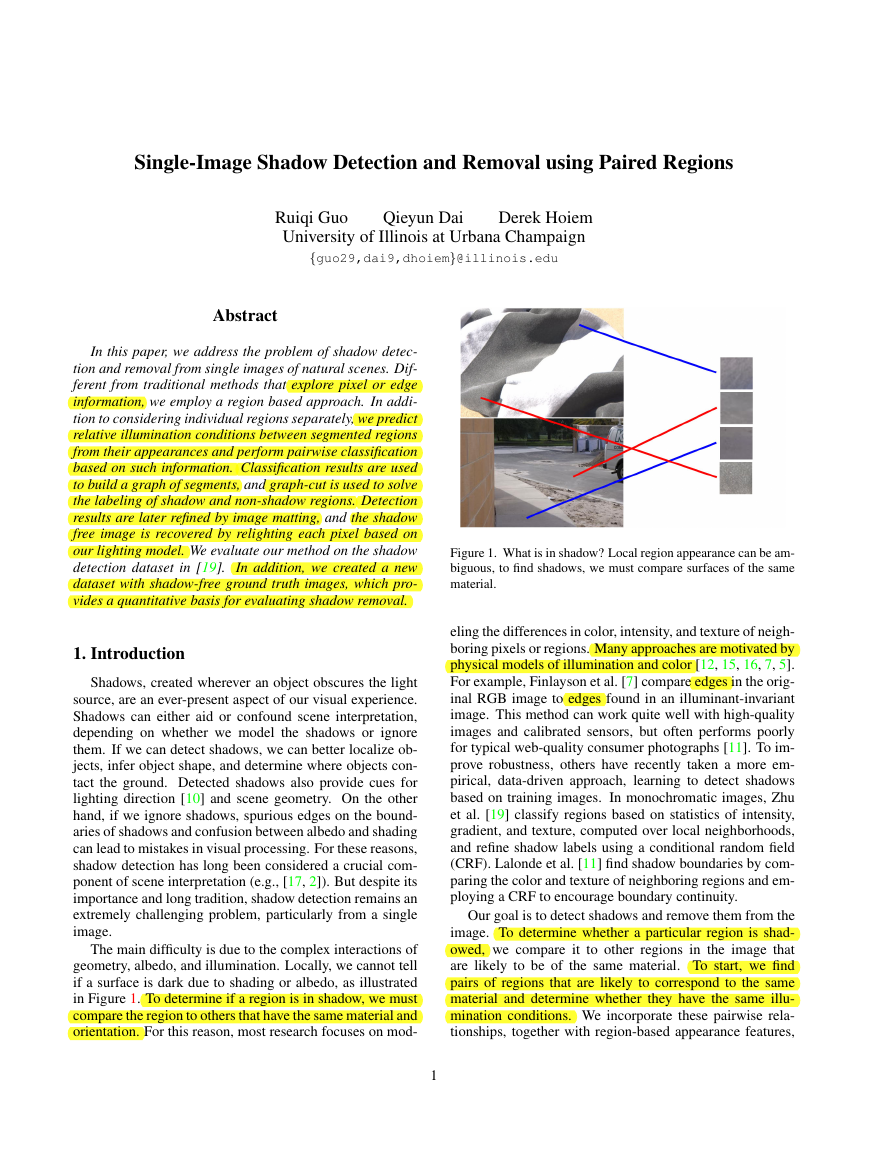
geometry, albedo, and illumination. Locally, we cannot tell
if a surface is dark due to shading or albedo, as illustrated
in Figure 1. To determine if a region is in shadow, we must
compare the region to others that have the same material and
orientation. For this reason, most research focuses on mod-
Figure 1. What is in shadow? Local region appearance can be am-
biguous, to find shadows, we must compare surfaces of the same
material.
eling the differences in color, intensity, and texture of neigh-
boring pixels or regions. Many approaches are motivated by
physical models of illumination and color [12, 15, 16, 7, 5].
For example, Finlayson et al. [7] compare edges in the orig-
inal RGB image to edges found in an illuminant-invariant
image. This method can work quite well with high-quality
images and calibrated sensors, but often performs poorly
for typical web-quality consumer photographs [11]. To im-
prove robustness, others have recently taken a more em-
pirical, data-driven approach, learning to detect shadows
based on training images. In monochromatic images, Zhu
et al. [19] classify regions based on statistics of intensity,
gradient, and texture, computed over local neighborhoods,
and refine shadow labels using a conditional random field
(CRF). Lalonde et al. [11] find shadow boundaries by com-
paring the color and texture of neighboring regions and em-
ploying a CRF to encourage boundary continuity.
Our goal is to detect shadows and remove them from the
image. To determine whether a particular region is shad-
owed, we compare it to other regions in the image that
are likely to be of the same material. To start, we find
pairs of regions that are likely to correspond to the same
material and determine whether they have the same illu-
mination conditions. We incorporate these pairwise rela-
tionships, together with region-based appearance features,
1
�
et al. [13], treating shadow pixels as foreground and non-
shadow pixels as background. Using the recovered shadow
coefficients, we calculate the ratio between direct light and
environment light and generate the recovered image by re-
lighting each pixel with both direct light and environment
light.
To evaluate our shadow detection and removal, we pro-
pose a new dataset with 108 natural scenes, in which ground
truth is determined by taking two photographs of a scene
after manipulating the shadows (either by blocking the di-
rect light source or by casting a shadow into the image).
To the best of our knowledge, our dataset is the first to en-
able quantitative evaluation of shadow removal on dozens
of images. We also evaluate our shadow detection on Zhu
et al.’s dataset of manually ground-truthed outdoor scenes,
comparing favorably to Zhu et al. [19].
The main contributions of this paper are (1) a new
method for detecting shadows using a relational graph of
paired regions; (2) an automatic shadow removal procedure
derived from lighting models making use of shadow mat-
ting to generate soft boundaries between shadow and non-
shadow areas; (3) quantitative evaluation of shadow detec-
tion and removal, with comparison to existing work; (4) a
shadow removal dataset with shadow free ground truth im-
ages. We believe that more robust algorithms for detecting
and removing shadows will lead to better recognition and
estimates of scene geometry.
2. Shadow Detection
To detect shadows, we must consider the appearance of
the local and surrounding regions. Shadowed regions tend
to be dark, with little texture, but some non-shadowed re-
gions may have similar characteristics. Surrounding regions
that correspond to the same material can provide much
stronger evidence. For example, suppose region si is similar
to sj in texture and chromaticity. If si has similar intensity
to sj, then they are probably under the same illumination
and should receive the same shadow label (either shadow or
non-shadow). However, if si is much darker than sj, then
si probably is in shadow, and sj probably is not.
We first segment the image using the mean shift algo-
rithm [4]. Then, using a trained classifier, we estimate the
confidence that each region is in shadow. We also find
same illumination pairs and different illumination pairs of
regions, which are confidently predicted to correspond to
the same material and have either similar or different illu-
mination, respectively. We construct a relational graph us-
ing a sparse set of confident illumination pairs. Finally, we
solve for the shadow labels y = {−1, 1}n (1 for shadow)
that maximize the following objective:
yi + α1
cdiff
ij
{i,j}∈Ediff
(yi − yj)
(1)
i=1
ij 1(yi = yj)
csame
cshadow
i
y
ˆy = arg max
− α2
{i,j}∈Esame
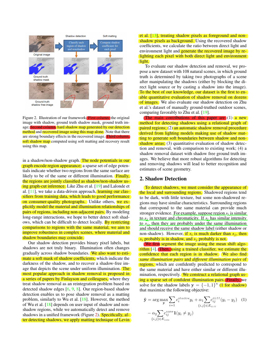
Figure 2. Illustration of our framework. First column: the original
image with shadow, ground truth shadow mask, ground truth im-
age; Second column, hard shadow map generated by our detection
method and recovered image using this map alone. Note that there
are strong boundary effects in the recovered image. Third column,
soft shadow map computed using soft matting and recovery result
using this map.
in a shadow/non-shadow graph. The node potentials in our
graph encode region appearance; a sparse set of edge poten-
tials indicate whether two regions from the same surface are
likely to be of the same or different illumination. Finally,
the regions are jointly classified as shadow/non-shadow us-
ing graph-cut inference. Like Zhu et al. [19] and Lalonde et
al. [11], we take a data-driven approach, learning our clas-
sifiers from training data, which leads to good performance
on consumer-quality photographs. Unlike others, we ex-
plicitly model the material and illumination relationships of
pairs of regions, including non-adjacent pairs. By modeling
long-range interactions, we hope to better detect soft shad-
ows, which can be difficult to detect locally. By restricting
comparisons to regions with the same material, we aim to
improve robustness in complex scenes, where material and
shadow boundaries may coincide.
Our shadow detection provides binary pixel labels, but
shadows are not truly binary.
Illumination often changes
gradually across shadow boundaries. We also want to esti-
mate a soft mask of shadow coefficients, which indicate the
darkness of the shadow, and to recover a shadow-free im-
age that depicts the scene under uniform illumination. The
most popular approach in shadow removal is proposed in
a series of papers by Finlayson and colleagues, where they
treat shadow removal as an reintegration problem based on
detected shadow edges [6, 9, 8]. Our region-based shadow
detection enables us to pose shadow removal as a matting
problem, similarly to Wu et al. [18]. However, the method
of Wu et al. [18] depends on user input of shadow and non-
shadow regions, while we automatically detect and remove
shadows in a unified framework (Figure 2). Specifically, af-
ter detecting shadows, we apply matting technique of Levin
�
i
ij
where cshadow
is the single-region classifier confidence
weighted by region area; {i, j} ∈ Ediff are different illu-
mination pairs; {i, j} ∈ Esame are same illumination pairs;
csame
are the area-weighted confidences of the
ij
pairwise classifiers; α1 and α2 are parameters; and 1(.) is
an indicator function.
and cdiff
In the following subsections, we describe the classifiers
for single regions (Section 2.1) and pairs of regions (Sec-
tion 2.2) and how we can reformulate our objective func-
tion to solve it efficiently with the graph-cut algorithm (Sec-
tion 2.3).
2.1. Single Region Classification
When a region becomes shadowed, it becomes darker
and less textured (see [19] for empirical analysis). Thus,
the color and texture of a region can help predict whether it
is in shadow. We represent color with a histogram in L*a*b
space, with 21 bins per channel. We represent texture with
the texton histogram provided by Martin et al. [14]. We
train our classifier from manually labeled regions using an
SVM with a χ2 kernel (slack parameter C = 1). We define
as the output of this classifier times ai, the pixel
cshadow
i
area of region i.
2.2. Pair-wise Region Relationship Classification
We cannot determine whether a region is in shadow by
considering only its internal appearance; we must compare
the region to others with the same material. In particular,
we want to find same illumination pairs, regions that are of
the same material and illumination, and different illumina-
tion pairs, regions that are of the same material but different
illumination. Differences in illumination can be caused by
direct light blocked by other objects or by a difference in
surface orientation. In this way, we can account for both
shadows and shading. Comparison between regions with
different materials is uninformative because they have dif-
ferent reflectance.
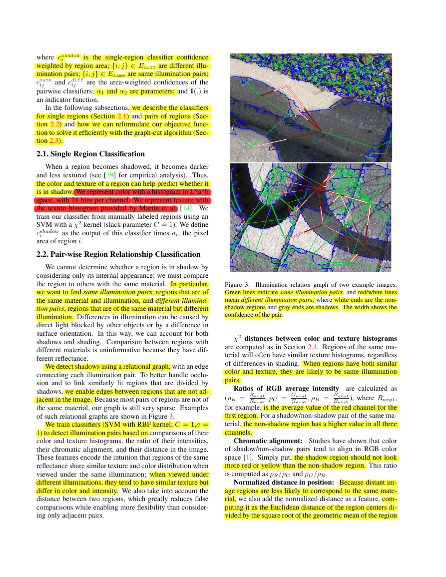
We detect shadows using a relational graph, with an edge
connecting each illumination pair. To better handle occlu-
sion and to link similarly lit regions that are divided by
shadows, we enable edges between regions that are not ad-
jacent in the image. Because most pairs of regions are not of
the same material, our graph is still very sparse. Examples
of such relational graphs are shown in Figure 3.
We train classifiers (SVM with RBF kernel; C = 1,σ =
1) to detect illumination pairs based on comparisons of their
color and texture histograms, the ratio of their intensities,
their chromatic alignment, and their distance in the image.
These features encode the intuition that regions of the same
reflectance share similar texture and color distribution when
viewed under the same illumination; when viewed under
different illuminations, they tend to have similar texture but
differ in color and intensity. We also take into account the
distance between two regions, which greatly reduces false
comparisons while enabling more flexibility than consider-
ing only adjacent pairs.
Figure 3.
Illumination relation graph of two example images.
Green lines indicate same illumination pairs, and red/white lines
mean different illumination pairs, where white ends are the non-
shadow regions and gray ends are shadows. The width shows the
confidence of the pair.
χ2 distances between color and texture histograms
are computed as in Section 2.1. Regions of the same ma-
terial will often have similar texture histograms, regardless
of differences in shading. When regions have both similar
color and texture, they are likely to be same illumination
pairs.
, ρG = Gavg1
Gavg2
Ratios of RGB average intensity are calculated as
(ρR = Ravg1
), where Ravg1,
Ravg2
for example, is the average value of the red channel for the
first region. For a shadow/non-shadow pair of the same ma-
terial, the non-shadow region has a higher value in all three
channels.
, ρB = Bavg1
Bavg2
Chromatic alignment: Studies have shown that color
of shadow/non-shadow pairs tend to align in RGB color
space [1]. Simply put, the shadow region should not look
more red or yellow than the non-shadow region. This ratio
is computed as ρR/ρG and ρG/ρB.
Normalized distance in position: Because distant im-
age regions are less likely to correspond to the same mate-
rial, we also add the normalized distance as a feature, com-
puting it as the Euclidean distance of the region centers di-
vided by the square root of the geometric mean of the region
�
ij
ij
We define csame
areas.
as the output of the classifier for same-
illumination pairs times √
aiaj, the geometric mean of the
region areas. Similarly, cdiff
is the output of the classi-
fier for different-illumination pairs times √
aiaj. Edges are
weighted by region area and classifier score so that larger
regions and those with more confidently predicted relations
have more weight. Note that the edges in Ediff are direc-
tional: they encourage yi to be shadow and yj to be non-
shadow. In both cases, the 100 most confident edges are
included if their classifier scores are greater than 0.6 (sub-
sequent experiments indicate that including all edges with
positive scores yields similar performance).
2.3. Graph-cut Inference
We can apply efficient and optimal graph-cut inference
by reformulating our objective function (Eq. 1) as the fol-
lowing energy minimization:
costunary
k
(yk) + α2
csame
ij
{i,j}∈Esame
1(yi = yj)
(2)
(yk) = − cshadow
yk − α1
k
cdiff
ij
{i=k,j}∈Ediff
yk
(3)
cdiff
+ α1
ij
{i,j=k}∈Ediff
yk.
k
ˆy = arg min
y
with
costunary
k
Because this is submodular (binary, with pairwise term en-
couraging affinity), we can solve for ˆy using graph cuts [3].
In our experiments, α1 = α2 = 1.
3. Shadow removal
Our shadow removal approach is based on a simple
shadow model where lighting consists of directed light and
environment light. We try to identify how much direct light
is occluded for each pixel in the image and relights the
whole image using that information. First, we use a mat-
ting technique to estimate a fractional shadow coefficient
value. Then, we estimate the ratio of direct to environmental
light, which together with the shadow coefficient, enables a
shadow-free image to be recovered.
3.1. Shadow model
In our illumination model, there are two types of light
sources: direct light and environment light. Direct light
comes directly from the source (e.g., the sun), while en-
vironment light is from reflections of surrounding surfaces.
Non-shadow areas are lit by both direct light and environ-
ment light, while for shadow areas, part or all of the direct
light is occluded. The shadow model can be represented by
the formula below.
Ii = (ti cosθi Ld + Le)Ri
(4)
where Ii is a vector representing the value for the i-th pixel
in RGB space. Similarly, both Ld and Le are vectors of
size 3, each representing the intensity of the direct light
and environment light, also measured in RGB space. Ri
is the surface reflectance of that pixel, also a vector of three
dimensions, each corresponding to one channel. θi is the
angle between the direct lighting direction and the surface
norm, and ti is a value between [0, 1] indicating how much
direct light gets to the surface. The equations in Section 3
for matrix computation refers to a pointwise computation,
except for the spectral matting energy function and its solu-
tion. When ti = 1, the pixel is in a non-shadow area, and
when ti = 0, the pixel is in an umbra, otherwise, the area
is in a penumbra (0 < ti < 1). For an shadow-free image,
every pixel is lit by both direct light and environment light
and can be expressed as:
Ishadow f ree
i
= (Ldcosθi + Le)Ri
We define ki = ti cos θi, which we will refer to ki as the
shadow coefficient for the i-th pixel in the rest of the paper;
ki = 1 for pixels in non-shadow regions.
3.2. Shadow Matting
The shadow detection procedure provides us with a bi-
nary shadow mask where each pixel i is assigned a ˆki
value of either 1 or 0. However, illumination often changes
gradually along shadow, and segmentation results are of-
ten inaccurate near the boundaries of regions. Using detec-
tion results as shadow coefficient values can create strong
boundary effects. To get more accurate ki values and get
smooth changes between non-shadow regions and recov-
ered shadow regions, we apply soft matting technique.
Given an image I, matting tries to separate the fore-
ground image F and background image B based on the fol-
lowing formulation.
Ii = γiFi + (1 − γi)Bi
Ii is the RGB value of the i-th pixel of the original image
I, and Fi and Bi are respectively the RGB value of the i-
th pixel of the foreground F and background image B. By
rewriting the shadow formulation given in (4) as:
Ii = ki(LdRi + LeRi) + (1 − ki)LeRi
an image with shadow can be seen as the linear combina-
tion of a shadow-free image LdR + LeR and a shadow im-
age LeR (R is a three dimensional matrix whose i-th entry
equals Ri), a formulation identical to that of image matting.
To solve the matting problem, we employ the spectral
matting algorithm from [13], minimizing the following en-
ergy function:
E(k) = kTLk + λ(k − ˆk)T D(k − ˆk)
where ˆk indicates the estimated shadow label (Section 2),
with ˆki = 0 being shadow areas and ˆki = 1 being non-
shadow. D is a diagonal matrix where D(i, i) = 1 when
�
the ki for the i-th pixel should agree with ˆki and 0 when the
ki value is to be predicted by the matting algorithm. In our
experiments, we set D(i, i) = 0 for pixels within a 5-pixel
distance of the detected label boundary, and D(i, i) = 1 for
all other pixels. L is the matting Laplacian matrix proposed
in [13], aiming to enforce smoothness over local patches.
In our experiments, a patch size of 3 × 3 is used.
The optimal k value is the solution to the following
sparse linear system:
(L + λD)k = λdˆk
where d is the vector comprising of elements on the diago-
nal of the matrix D. In our experiments, we empirically set
λ to 0.01.
3.3. Ratio Calculation and Pixel Relighting
Based on our shadow model, we can relight each pixel
using the calculated ratio and k value. The new pixel value
is given by:
Ishadow f ree
i
= (Ld + Le)Ri
= (kiLd + Le)Ri
Ld + Le
kiLd + Le
=
r + 1
kir + 1
Ii
(5)
(6)
(7)
is the ratio between direct light and environ-
where r = Ld
Le
ment light and Ii is the intensity of the i-th pixel in the orig-
inal image. For each channel, we recover the pixel value
separately. We now show how to recover r from detected
shadows and matting results.
To calculate the ratio between direct light and environ-
ment light, our model checks for adjacent shadow/non-
shadow pairs along the shadow boundary. We believe
these patches are of the same material and reflectance. We
also assume direct light and environment light is consistent
throughout the image. Based on the lighting model, for two
pixels with the the same reflectance, we have:
Ii = (kiLd + Le)Ri
Ij = (kjLd + Le)Rj
with Ri = Rj.
From the above equations, we can arrive at:
r =
Ld
Le
=
Ij − Ii
Iikj − Ijki
To estimate r, we sample patches from shadow/non-shadow
pairs and vote for values of r based on average RGB inten-
sity and k values within the pairs of patches. Votes in the
joint RGB ratio space are accumulated with a histogram,
and the center value of the bin with the most votes is used
for r. The bin size is set to 0.1, and the patch size is 4 × 4
pixels.
4. Experiments and Results
In our experiments, we evaluate both shadow detection
and shadow removal results. For shadow detection, we mea-
sure how explicitly modeling the pairwise region relation-
ship affects detection results and how well our detector can
generalize cross datasets. For shadow removal, we evalu-
ate the results quantitatively on our dataset by comparing
the recovered image with the shadow-free ground truth and
show qualitative results on both our dataset and the UCF
shadow dataset [19].
4.1. Dataset
Our shadow detection and removal methods are evalu-
ated on the UCF shadow dataset [19] and our proposed new
dataset. Zhu et al. made available a set of 245 images they
collected themselves and from Internet, with manually la-
beled ground truth shadow masks.
Our training set consists of 32 images with manually an-
notation of shadow regions and pairs illumination condi-
tions between regions. Our test set contains 76 image pairs,
collected from common scenes or objects under a variety
of illumination conditions, both indoor and outdoor. Each
pair consists of a shadowed image (the input to the algo-
rithm) and a ground truth image where every pixel in the
image has the same illumination. For 46 image pairs, we
taken one image with shadow and then another shadow-free
ground truth image by removing the source of the shadow.
The light sources for both images remain the same. One
disadvantage of this approach is that it does not include self
shadows of objects. To account for that, we collect another
set of 30 images where shadows are caused by objects in
the scene. To create an image pair for this set of images, we
block the light source so that the whole scene is in shadow.
We automatically generate the ground truth shadow mask
by thresholding the ratio between the two images in a pair.
This approach is more accurate and robust than manually
annotating shadow regions.
4.2. Shadow Detection Evaluation
Two sets of experiments are carried out for shadow de-
tection. First, we try to compare the performance when
using only the unary classifier, only the pairwise classi-
fier, and both combined. Second, we conduct cross dataset
evaluation, training on one dataset and testing on the other.
The per pixel accuracy on the testing set is reported in Fig-
ure 4(c) and the qualitative results are shown in Figure 5.
4.2.1 Comparison between unary and pairwise infor-
mation
Using only unary information, the performance on the UCF
dataset is 87.5%, versus a 83.4% achieved by classifying
everything to non-shadow, and 88.7% reported in [19].
Different from our approach which makes use of color in-
formation,
[19] conducts shadow detection on gray scale
�
images. By combining unary information with pairwise in-
formation, we achieved an accuracy of 90.0%. Note that
we are using a simpler set of features and simpler learning
method than [19].
The pairwise illumination relations are especially impor-
tant on our dataset. Using them, the overall accuracy in-
creases by more than 8%, and 50% more shadow areas are
detected than with the single region classifier.
4.2.2 Cross dataset evaluation
The result in Figure 4(d) indicate that our proposed detec-
tor can generalize across datasets. This is especially no-
table since the two datasets are very different in nature, with
[19] containing more large scale scenes and hard shadows.
As shown in Figure 4(d), the unary and pairwise classifiers
trained on [19] performs well on both datasets. This is un-
derstandable since their dataset is more diverse and contains
more training images.
4.3. Shadow Removal Evaluation
To evaluate shadow free image recovery, we used as
measurement the root mean square error (RMSE) in L*a*b
color space between the ground truth shadow free image
and the recovered image, which is designed to be locally
perceptually uniform. We evaluate our results on the whole
image as well as shadow and non-shadow regions sepa-
rately.
The quantitative evaluation is performed on the subset
of images with ground truth shadow free image (a total of
46 images). Shadow/non-shadow regions are given by the
ground truth shadow mask introduced in the previous sec-
tion. As shown in Table 4(e), our shadow removal proce-
dure based on image matting yields results that are percep-
tually close to ground truth.
We show results overall and individually for shadow
and non-shadow regions (according to the binary ground
truth labels). The “non-shadow” regions may contain light
shadows, so that error between original and ground truth
shadow-free images is not exactly zero for these regions.
To show that matting helps achieve smooth boundaries, we
also compare the recovery results using only the detected
hard mask. We also show results using soft matte generated
from the ground truth hard mask, which provides a more
accurate evaluation of the recovery algorithm.
The qualitative results for shadow removal are shown in
Figure 5: 5(a) shows the detection and removal results on
the UCF shadow dataset [19]; 5(b) demonstrates results on
our dataset; and 5(c) is an example where our shadow de-
tector successfully detects the self-shadow on the box. An
interesting failure example is shown in Fig. 5(d) where the
darker parts of the checkerboard are paired with the lighter
parts by the pairwise detector and thus removed in the re-
covery stage.
5. Conclusion and Discussion
In conclusion, we proposed a novel approach to de-
tect and remove shadows from a single still image. For
shadow detection, we have shown that pairwise relation-
ship between regions provides valuable additional informa-
tion about illumination condition of regions, compared with
simple appearance-based models. We also show that by ap-
plying soft matting to the detection results, the lighting con-
ditions for each pixel in the image are better reflected, es-
pecially for those pixels on the boundary of shadow areas.
Our conclusions are supported by quantitative experiments
on shadow detection and removal in Figure 4(c) and 4(e).
Currently our detection method relies on the initial seg-
mentation which may group soft shadows with non-shadow
regions. In our model, we do not differentiate whether illu-
mination changes are caused by shadows or shading due to
orientation discontinuities, such as building walls.
To further improve detection, we could incorporate more
sophisticated features, such as those in Zhu et al. [19]. We
could also incorporate geometry estimates into our detec-
tion framework, as in Lalonde et al. [11], which could help
to remove false pairings between regions and to indicate the
source of the shadow. We will make available our dataset
and code, which we hope will facilitate the use of shadow
detection and removal in scene understanding.
Acknowledgements
This work was supported in part by the National Sci-
ence Foundation under IIS-0904209 and by a Google Research
Award.
References
[1] M. Baba and N. Asada. Shadow removal from a real picture.
In SIGGRAPH, 2003. 3
[2] H. Barrow and J. Tenenbaum. Recovering intrinsic scene
characteristics from images. In Comp. Vision Systems, 1978.
1
[3] Y. Boykov, O. Veksler, and R. Zabih. Fast approximate en-
ergy minimization via graph cuts. PAMI, 23(11):1222–1239,
2001. 4
[4] D. Comaniciu and P. Meer. Mean shift: A robust approach
toward feature space analysis. PAMI, 24(5):603–619, 2002.
2
[5] G. D. Finlayson, M. S. Drew, and C. Lu. Entropy minimiza-
tion for shadow removal. IJCV, 85(1):35–57, 2009. 1
[6] G. D. Finlayson, S. D. Hordley, and M. S. Drew. Remov-
ing shadows from images using retinex. In Color Imaging
Conference. IS&T - The Society for Imaging Science and
Technology, 2002. 2
[7] G. D. Finlayson, S. D. Hordley, C. Lu, and M. S. Drew. On
the removal of shadows from images. PAMI, 28:59–68, Jan
2006. 1
[8] C. Fredembach and G. Finlayson. Hamiltonian path-based
shadow removal. In BMVC, volume 2, pages 502–511, Ox-
ford, U.K., 2005. 2
[9] C. Fredembach and G. D. Finlayson. Fast re-integration of
In Color Imaging Conference, pages
shadow free images.
�
Our dataset (unary)
Shadow(GT)
Non-shadow(GT)
Our dataset (unary+pairwise)
Shadow(GT)
Non-shadow(GT)
UCF (unary)
Shadow(GT)
Non-shadow(GT)
UCF (unary+pairwise)
Shadow(GT)
Non-shadow(GT)
UCF (Zhu et al. [19])
Shadow(GT)
Non-shadow(GT)
0.531
0.909
0.291
0.943
Shadow Non-shadow
0.469
0.091
Shadow Non-shadow
0.709
0.057
Shadow Non-shadow
0.515
0.053
Shadow Non-shadow
0.750
0.070
Shadow Non-shadow
0.639
0.067
0.361
0.934
0.485
0.947
0.250
0.930
(a) Detection confusion matrices
(b) ROC Curve on UCF dataset
BDT+BCRF [19]
Our method
Unary SVM
Pairwise SVM
Unary SVM + adjacent Pairwise
Unary SVM + Pairwise
UCF shadow dataset Our dataset
0.887
0.875
0.673
0.897
0.900
-
0.796
0.794
0.872
0.883
(c) Shadow detection evaluation (per pixel accuracy)
pixel accuracy on UCF dataset
Training source
Unary UCF
Unary UCF,Pairwise UCF
Unary UCF,Pairwise Ours
Unary Ours
Unary Ours,Pairwise UCF
Unary Our,Pairwise Our
0.875
0.900
0.879
0.680
0.752
0.794
pixel accuracy on our dataset
0.818
0.864
0.884
0.796
0.861
0.883
(d) Cross dataset shadow detection
Original No matting Automatic matting Matting with Ground Truth Mask
Region Type
Overall
Shadow regions
Non-shadow regions
13.7
42.0
4.6
8.7
18.3
5.6
8.3
16.7
5.6
6.4
11.4
4.8
(e) Shadow removal evaluation on our dataset(pixel intensity RMSE)
Figure 4. (a) Confusion matrices for shadow detection. (b) ROC Curve on UCF dataset. (c) The average per pixel accuracy on both dataset.
(d) cross dataset tasks, testing the detector trained on one dataset on another one. (e) The per pixel RMSE for shadow removal task. First
column shows the error when no recovery is performed; the second column is when detected shadow masks are directly used for recovery
and no matting is applied; the third column is the result of using soft shadow masks generated by matting; the last column shows the result
of using soft shadow masks generated from ground truth mask.
117–122. IS&T - The Society for Imaging Science and Tech-
nology, 2004. 2
[10] J.-F. Lalonde, A. A. Efros, and S. G. Narasimhan. Estimating
natural illumination from a single outdoor image. In ICCV,
2009. 1
[11] J.-F. Lalonde, A. A. Efros, and S. G. Narasimhan. Detect-
In
ing ground shadows in outdoor consumer photographs.
ECCV, 2010. 1, 2, 6
[12] E. H. Land, John, and J. Mccann. Lightness and retinex the-
ory. Journal of the Optical Society of America, pages 1–11,
1971. 1
[13] A. Levin, D. Lischinski, and Y. Weiss. A closed-form solu-
tion to natural image matting. PAMI, 30(2):228–242, 2008.
2, 4, 5
[14] D. R. Martin, C. Fowlkes, and J. Malik. Learning to detect
natural image boundaries using local brightness, color, and
�
(a)
(b)
(c)
(d)
Figure 5.
(a)Detection and recovery results on UCF dataset [19]. These results show that our detection and recovery framework also
works well in complicated scenes. (b) Detection and recovery results on our dataset. (c) Example of detection and recovery on scenes with
self-shadow. The self-shadow is correctly detected by our detector. (d) Failure example. The darker parts of the chessboard are mistakenly
detected as shadow and as a result, removed in the recovery process.
texture cues. PAMI, 26(5):530–549, 2004. 3
[15] B. A. Maxwell, R. M. Friedhoff, and C. A. Smith. A bi-
illuminant dichromatic reflection model for understanding
images. In CVPR, 2008. 1
[16] S. G. Narasimhan, V. Ramesh, and S. K. Nayar. A class of
photometric invariants: Separating material from shape and
illumination. In ICCV, 2003. 1
[17] D. L. Waltz. Generating semantic descriptions from draw-
ings of scenes with shadows. Technical report, Cambridge,
MA, USA, 1972. 1
[18] T.-P. Wu, C.-K. Tang, M. S. Brown, and H.-Y. Shum. Natural
shadow matting. ACM Trans. Graph., 26(2), 2007. 2
[19] J. Zhu, K. G. G. Samuel, S. Masood, and M. F. Tappen.
Learning to recognize shadows in monochromatic natural
images. In CVPR, 2010. 1, 2, 3, 5, 6, 7, 8
�



 2023年江西萍乡中考道德与法治真题及答案.doc
 2012年重庆南川中考生物真题及答案.doc
 2013年江西师范大学地理学综合及文艺理论基础考研真题.doc
 2020年四川甘孜小升初语文真题及答案I卷.doc
 2020年注册岩土工程师专业基础考试真题及答案.doc
 2023-2024学年福建省厦门市九年级上学期数学月考试题及答案.doc
 2021-2022学年辽宁省沈阳市大东区九年级上学期语文期末试题及答案.doc
 2022-2023学年北京东城区初三第一学期物理期末试卷及答案.doc
 2018上半年江西教师资格初中地理学科知识与教学能力真题及答案.doc
 2012年河北国家公务员申论考试真题及答案-省级.doc
 2020-2021学年江苏省扬州市江都区邵樊片九年级上学期数学第一次质量检测试题及答案.doc
 2022下半年黑龙江教师资格证中学综合素质真题及答案.doc