Robotics and Autonomous Systems 82 (2016) 1–14
Contents lists available at ScienceDirect
Robotics and Autonomous Systems
journal homepage: www.elsevier.com/locate/robot
Unified framework for path-planning and task-planning for
autonomous robots
Pablo Muñoz∗, María D. R-Moreno, David F. Barrero
Universidad de Alcalá, Departamento de Automática Campus Universitario, Ctra. Madrid-Barcelona, Km. 33, 600, 28871 Alcalá de Henares, Spain
h i g h l i g h t s
• A planner for mobile robotics applications is proposed.
• Integrating task-planning and path-planning provides several advantages.
• Using specific and domain independent heuristics improves the solutions generated.
a r t i c l e
i n f o
a b s t r a c t
Article history:
Received 30 January 2015
Received in revised form
4 April 2016
Accepted 22 April 2016
Available online 11 May 2016
Keywords:
Task-planning
Path-planning
Autonomy
Robot control architectures
Most of the robotic systems are designed to move and perform tasks in a variety of environments. Some
of these environments are controllable and well-defined, and the tasks to be performed are generally
everyday ones. However, exploration missions also enclose hard constraints such as driving vehicles to
many locations in a surface of several kilometres to collect and/or analyse interesting samples. Therefore,
a critical aspect for the mission is to optimally (or sub-optimally) plan the path that a robot should follow
while performing scientific tasks. In this paper, we present up2ta, a new AI planner that interleaves path-
planning and task-planning for mobile robotics applications. The planner is the result of integrating a
modified PDDL planner with a path-planning algorithm, combining domain-independent heuristics and
a domain-specific heuristic for path-planning. Then, up2ta can exploit capabilities of both planners to
generate shorter paths while performing scientific tasks in an efficient ordered way. The planner has been
tested in two domains: an exploration mission consisting of pictures acquisition, and a more challenging
one that includes samples delivering. Also, up2ta has been integrated and tested in a real robotic platform
for both domains.
© 2016 Elsevier B.V. All rights reserved.
1. Introduction
Nowadays, most of the robotic systems that are being designed
have to move and perform tasks in a variety of environments.
In order to do that, they have to avoid obstacles, find a collision
free trajectory, and plan tasks. Some of these systems aim to help
with ordinary, but tedious tasks. Generally, they move in known
surfaces and the number of decisions is usually limited such as
night surveillance tasks.
However, new science missions such as the two main missions
ExoMars and MARS Sample Return (part of the Aurora program
of the European Union Council of Research) will require more
capable systems to achieve the goals that they are designed for.
∗ Corresponding author.
E-mail addresses: pmunoz@aut.uah.es (P. Muñoz), mdolores@aut.uah.es
(M.D. R-Moreno), david@aut.uah.es (D.F. Barrero).
http://dx.doi.org/10.1016/j.robot.2016.04.010
0921-8890/© 2016 Elsevier B.V. All rights reserved.
Mobility and science capabilities of the rovers are increasing,
which require more powerful tools to assist on-ground operators
and autonomous capabilities for the rovers. In previous missions,
optimality in the path followed by the rover was not a difficult task
due to the short distances they could travel per day. However, a
critical aspect in future missions is to optimally (or sub-optimally)
plan the path that a robot should follow while performing scientific
tasks. In addition, improvements for such domains can also be
incorporated into commercial robotic applications, e.g. performing
inventory tasks in a large warehouse or autonomous logistics
domains [1].
In this direction, the paper presents some of the results
obtained within the Ph.D. program on the topic of Cooperative
Systems for Autonomous Exploration Missions supported by ESA.
Particularly, we are pursuing autonomous navigation with a
rover for an exploration domain with several scientific targets
along a known terrain. To face this problem, we initially had
a complex deliberative model expressed in Planning Domain
�
2
P. Muñoz et al. / Robotics and Autonomous Systems 82 (2016) 1–14
Definition Language (PDDL) [2] in which path-planning and task-
planning were solved with a PDDL planner. This solution was
very limited in (i) the map size because the planner only solved
small grids in a reasonable time, and (ii) the quality of path
generated because the planner generated suboptimal paths that
were impossible to improve by using recent research advantages
on path-planning algorithms. A second approach was to partially
detach path-planning and task-planning. Before the search process
starts, it is possible to include in the PDDL model a visibility
graph with connections between tasks, which is generated using
a path-planning algorithm. Then, the PDDL planner can obtain a
feasible solution to achieve all tasks. Finally, the path-planning
algorithm generates paths for the movements between each pair
of locations in the plan. However, in our experiments we observed
that solutions were not optimal. This was because of the domain
independent heuristic employed by the task-planner. Considering
a movement in the same way as other actions (e.g. take picture)
leads to not properly consider the distance between tasks.
For this reason, we have developed an Artificial Intelligence
(AI) planner that integrates capabilities of path-planning and
task-planning. The main idea is to take advantage of path-
planning heuristics and merge them with domain independent
heuristics to generate better solutions in robotic domains. The
proposed planner, called Unified Path-Planning and Task-Planning
Architecture (up2ta), is able to plan paths considering the shortest
path while performing scientific tasks in an efficient ordered way.
A PDDL planner is responsible of ordering the tasks while a path-
planning algorithm searches for the route between tasks. In up2ta,
these planners are highly coupled, allowing to merge the heuristics
of both planners in order to provide better solutions for mobile
robotics domains. We perform an experimental evaluation of our
planner on two classical exploration domains: pictures acquisition
and samples delivering. In addition, up2ta is currently deployed as
the deliberative layer of the Model-Based Autonomous Controller
(MoBAr) [3,4], which has been also used in our evaluation.
The next section reviews those heuristic algorithms for path-
planning that are used within our planner. Section 3 presents a
brief description of heuristic planners in the state-of-the-art, with
a special focus on the ff planner that we use in our integration.
Section 4 defines approaches that interleave task-planning and
motion/path-planning. Section 5 describes our initial attempt to
solve problems without a heuristic integration schema. Section 6
introduces two application domains that are then used in an
experimental evaluation, which is shown in Section 8. Section 9
presents some conclusions.
2. Path-planning review
In this section, we review the most common path-planning
algorithms and their features. In particular, we focus on heuristic
search algorithms applied to path-planning since we use those in
our integration.
2.1. Representation and notation
In classical path-planning, the environment is usually repre-
sented as a two-dimensional uniform grid with blocked and un-
blocked cells [5]. There are two types of representations: the node
can be in the centre of the cell (centre node representation) or the
node can be on the corner of the cell (corner node representation).
In both cases, a valid path is the one that starts from the initial node
and reaches the goal without crossing a blocked cell.
From now on, consider a node p as a random node, and s
and g as the initial and goal nodes respectively. Each node p is
defined by its coordinate pair (xp, yp). A solution has the form
(p1, p2, . . . , pn−1, pn) where p1 = s and goal pn = g. For each node
p we require the following information:
• predecessors(p): the predecessor node of p. It is mandatory that
the straight line between p and its predecessors does not cross
blocked cells.
• successors(p): a list of nodes that are reachable from p. The
predecessors of each node t in the list is p. Therefore, if
predecessors(t) = p ⇒ t ∈ successors(p).
• G(p): the length of the path from s to p.
• H(p): the heuristic value of p, i.e., an estimation of the distance
from p to g. Typically, the A* algorithm [6] uses the Octile
distance, while Theta* [7] uses the Euclidean distance.
2.2. Heuristic path-planning algorithms
A path-planning problem can be represented as a search
tree over grids. This representation has been widely discussed.
Algorithms such as A* allow us to quickly find routes at the expense
of an artificial restriction of direction changes of π /4. A* Post
Smoothed (A*PS) [8] tries to smooth the path obtained by A* in a
post-processing step. Therefore, the resulting path may be shorter
than the original, but has higher running time. If A* finds a path,
the smooth process checks the line of sight between every node
and the successor’s successor node, removing intermediate nodes
when possible. Also, there have been some improvements such
as its application to non-uniform costs setting in Field D* [9], or
more recently Theta* [7], which aims to remove the restriction on
direction changes that A* generates. Both algorithms use the same
evaluation function as in Eq. (1).
F(p) = G(p) + H(p).
(1)
The main difference between A* and Theta* [7] is that the
former only allows that the predecessors of a node is its
predecessor, while in the latter the predecessors of a node can be
any node. Usually, path-planning algorithms compliant with this
property (i.e. predecessors(t) = p ⇒ t ∈ successors(p) is no
longer mandatory) are called any-angle path-planning algorithms.
This property allows Theta* to find shorter paths with fewer
turns compared to A*. However, this improvement implies a
higher computational cost due to additional operations performed
during the nodes expansion process. These algorithms work on
fully observable environments except Field D* that can deal with
partially observable environments applying a replanning scheme.
From the Theta* algorithm, some effort has been performed in
order to improve its performance such as Incremental Phi* [10]
that takes into consideration the free-space assumption and angle
ranges computation to provide a speed-up of approximately one
order of magnitude with respect to Theta*; or Lazy Theta* [11] that
delays the computation of the line of sight checking (decreasing
the number of checks), and improves the performance in order to
deal with 3D cubic environments.
The Smooth Theta* (S-Theta*) [12] algorithm, developed from
Theta*, aims to reduce the amount of turns that the robot should
perform to reach the goal. The motivation is that robots could
require more time when turning, although is not desirable to
rotate big angles in soft terrains. The S-Theta* algorithm considers
early in the search process those nodes that follow the current
heading of the robot. Then, the evaluation function of A* or Theta* is
modified by adding a third parameter as in Eq. (2), which evaluates
the direction of the successor node with respect to the current
predecessors’ position and the goal node.
F(p) = G(p) + H(p) + α(p).
(2)
This means that, at the beginning of the search process the
algorithm tries to follow the line connecting the initial node
to the goal node. That is, the shortest route, if there are no
obstacles. When the initial direction needs to be changed because
of an obstacle in the path, the algorithm expands nodes taking
�
P. Muñoz et al. / Robotics and Autonomous Systems 82 (2016) 1–14
3
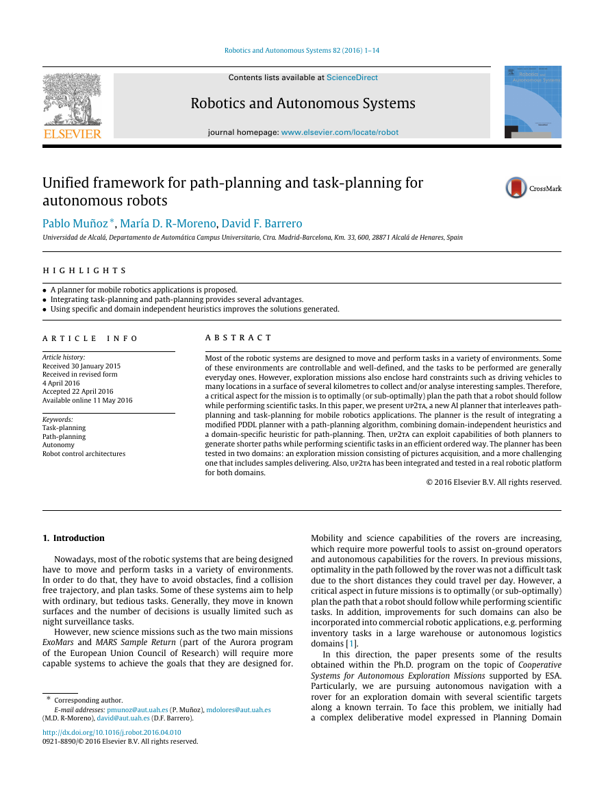
Fig. 1. α values with an obstacle in the current direction.
into consideration both the path length and the heading change
necessary to reach the successors. In this way, the search continues
towards a path with less amplitude turns, but it may obtain a
bit longer paths. This behaviour makes that S-Theta* can perform
heading changes at any point of the map, not only at the corners of
the obstacles as Theta* does. Fig. 1 shows the α value for nodes
r and t, which can be expanded when there is an obstacle q on
the current direction. We use the △ptg and △prg triangles to
compute α(t) and α(r), where p = predecessors(q) and (r, t) ∈
successors(q). Since the value of α(t) is lower than α(r), S-Theta*
will expand t. Conversely, Theta* would expand r.
In the same way, if we consider the α(p) value of a node as part
of the heuristic function instead of using it in the cost function, the
result is a path-planning algorithm that has a greedy behaviour.
This means that the algorithm tries to follow the straight line
between the initial and goal points s and g as a result of the
modified heuristic, which computes α(p) as the angle formed by
the triangle △spg for any node p.
Muñoz and R-Moreno [13] applied this technique to the A*PS
and Theta* algorithms. They showed that the modified heuristic
required less time and memory to obtain a path, but increased
its length with respect to Theta*. This is due to the number of
expanded nodes: algorithms using this heuristic expand fewer
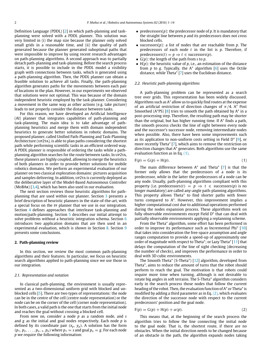
nodes than using their original ones. Fig. 2 shows a small example
of A* and the path and nodes expanded using the Octile distance,
and A* using α(p) as part of the heuristic function (presented
as Greedy-A*). It is also possible to deal with the resulting path
length, the search runtime, and the memory required using a
factor in order to weight the value of the α(p) function. Since the
heuristic computation is the only modification in the algorithm,
it is guaranteed that if there is a path between two nodes, the
algorithm will find it.
3. Heuristic search planners
Heuristic search planners use heuristic functions H(s) to find a
sequence of actions that reaches the goal from the initial state [14].
Heuristic functions are commonly generated by simplifying
the original problem. This is known as relaxation. A common
relaxation-based heuristic in planning is the delete relaxation,
which consists of ignoring delete effects. Considering a delete
relaxation problem, the estimated cost H+(s) from any state s to
the goal state can be seen as a lower bound of the optimal cost H∗(s)
for the original problem. As a result, the delete relaxation heuristic
H+(s) can be used as a heuristic for solving the original problem.
Fig. 2. Greedy-A* search for path-planning versus A*.
The additive and max heuristics are examples of relaxation-based
heuristics. In particular, the additive heuristic, Hadd(s), estimates
the cost of achieving a proposition p from a state s as the minimum
cost among all the actions a that produce p. Such cost is defined as
the sum of the cost of the individual preconditions of a. The max
heuristic, Hmax(s), estimates the cost of achieving a proposition p
from a state s as the minimum cost among all the actions a that
produce p. Such cost is defined as the maximum cost among all
preconditions of a.
Another relaxed-based heuristic is the high-order heuristic,
Hm(s) [15], which computes estimates of costs for sets of m
propositions from the initial state. The Pattern Databases (PDB)
heuristic [16] abstracts some variables of the problem, mapping
states of the original state space into the abstracted space in a way
that all states match the abstract space. The Hmax(s), Hm(s), and
PDB heuristics are admissible and, therefore, they can be used in an
A* algorithm for optimal planning. On the other hand, the Hadd(s)
is not admissible, but it has shown to be compelling in practice.
Recently, new search enhanced techniques such as helpful
actions [17], preferred operator [18], deferred evaluation [19],
and landmarks [20] have been developed to speed up the search.
However, in the last few years landmark detection algorithms
have been studied by the planning community to develop new
techniques to find and order landmarks [21].
There is a number of relevant heuristic planners that have
shown good performance in recent International Planning Compe-
titions (IPC). Some of them were initially considered candidates for
being used in the task-planning side of an autonomous controller
(MoBAr in our case) such as Fast Downward [18] or LAMA [22].
These two planners use finite-domains rather than binary state
variables. LAMA is currently one of the best-performing sequen-
tial planners. Another IPC winner is OPTIC [23], a temporal POP-
based planner that outperforms some IPC5 planners on problems
that deal with goal deadlines.
Recent planners can deal with complex domains that include
temporal constraints or preferences [24,25]. However, we have
decided to use the well-known ff [17] planner in our integration.
It was the winner of some competitions in the past. It is written
in C, making it very compact and fast, suitable for real robots
applications when the CPU is limited. Some newer planners such
as Metric-ff [26] and SGPlan [27] rely on ff. Therefore, it seems to
be possible that we can integrate our modifications without much
effort in ff-based planners. Since the aim of the paper is to evaluate
�
4
P. Muñoz et al. / Robotics and Autonomous Systems 82 (2016) 1–14
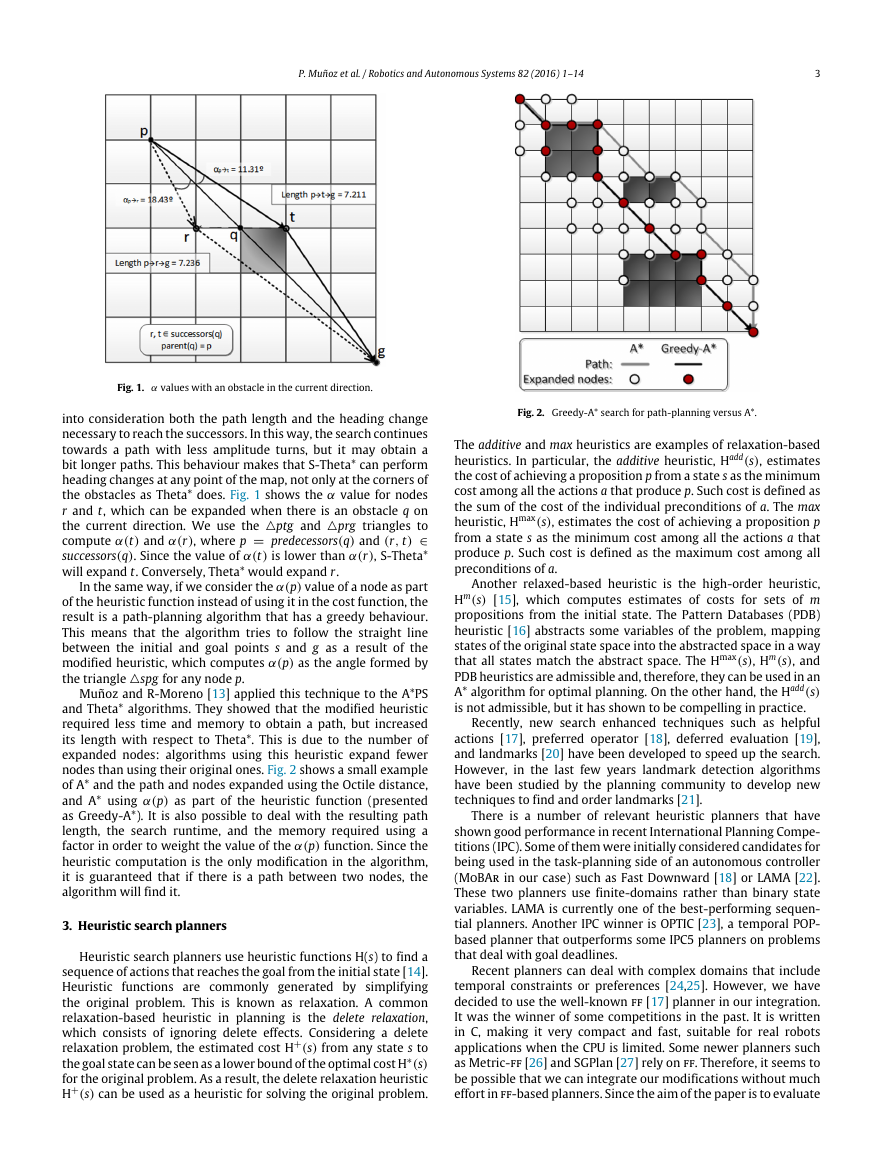
Fig. 3. ff general structure.
the integration between a path-planning heuristic and a domain-
independent heuristic provided by a task-planner, ff seems to be
good enough for our purposes without requiring some engineering
effort to made the integration. Newer planners are usually more
complex to be modified due to external modules, lexical analysers,
among others.
The ff planner is based on a relaxed planning graph. In general, a
planning graph is a directed graph composed of two types of nodes
distributed on several levels. Starting at level 0, the even levels
contain information about the propositions that are reached—fact
layers. The odd levels contain actions whose preconditions are
present at the previous level—action layers. The edges represent
the preconditions and effect relations (positive (add), negative
(del) and conditions that are maintained without executing any
action (no-op)) between facts and actions. Since delete relaxation
is assumed, a relaxed planning graph does not deal with negative
edges. Fig. 3 shows the ff architecture. This architecture is
implemented by three main modules that are summarized next.
• The Analysis and Processing module analyses and processes all
the information that comes from the domain and the problem.
• The Heuristic Computation module calculates the cost of
applying a determined node in the search process. The heuristic
used in ff is based on the number of actions or length in
an explicit solution from a relaxed-plan graph algorithm. The
length of the solution (that is, the number of actions) is taken
as an estimation of how far the goal is from the current state.
When calculating the number of actions, the heuristic always
prefers the no-ops against actions since they count as zero.
• The Search module directly depends on the heuristic compu-
tation. ff uses two search algorithms in combination with the
mentioned heuristic. First, ff uses Enforced Hill Climbing; when
a local minimum is encountered, breadth-first search is used
until a state with a strictly better heuristic is found; if breadth-
first fails, ff restarts to Best First Search (BFS). BFS is similar to
the A* algorithm explained in the previous section, with the dif-
ference that nodes are sorted according to their heuristic value.
4. Integration of task-planning and path-planning
Traditionally, task-planning and motion/path-planning prob-
lems were covered by separating both problems, i.e., high-level
task modelling ignores low-level constraints. This simplification
results in inefficient or even infeasible solutions. Then, works that
integrate task-planning and motion/path-planning to solve prob-
lems such as object manipulation or mobile robotics domains have
been reported in the literature, providing better solutions. We can
mention work done by Zacharias et al. [28], in which a two-arm
humanoid robot must manipulate objects on a table. The partic-
ular problem addressed is how to automatically rearrange and
manipulate objects without collisions. This is done by using a
motion-planner to compute trajectories, and a task-planner to pro-
vide the grasping operations that achieve a free-obstacle configu-
ration.
In this direction, Cambon et al. implemented the aSyMov
planner [29], which integrates Metric-ff for task-planning and
Probabilistic RoadMaps (PRM) [30] for motion-planning. For the
integration, both planners share a geometric representation of the
position of the robots, obstacles, and objects in the environment.
The plan extraction is guided by a task-planner, which initially
provides a solution for a problem in which all motion paths are
valid (i.e. no obstacles are considered). Then, a motion-planner
checks if it is possible to achieve the goals. Selection of actions is
guided by a cost function that adds (i) the number of times that an
action fails due to infeasible paths, and (ii) the heuristic computed
by the task-planner. When there are no valid paths to achieve a
goal, the motion-planner updates the geometrical information of
the task-planner, which must generate a new plan. Finally, when
a valid plan is generated, an improvement process is executed
with the aim of optimizing the planned paths while attempting to
parallelize actions in multi-robots domains.
The I-TMP algorithm [31] uses a motion-planning algorithm (a
PRM) to determine trajectory constraints for a logical description
of the tasks to perform. Such tasks are encoded in a formal language
similar to PDDL and solved with and integrated planner that
interleaves task and motion-planning. This planner shows a good
performance for planning the navigation of legged robots.
The SAHTN algorithm [32] is designed to deal with pick-
and-place domains for robots equipped with robotic arms.
The algorithm implements a hierarchy from Hierarchical Task
Networks (HTN) for task-planning to Rapidly-exploring Random
Trees (RRT) [33] for low-level actions (i.e. arm movement). In
this way, the hierarchy specifies a set of high-level actions that
can be refined until low-level movements. For each movement, a
reachable state space is produced that can be reused for different
objects. By doing this, the associated search cost is reduced and,
therefore, avoids infeasible solutions for the higher level.
Some of the above-mentioned approaches combine task-
planning and motion-planning in the search process in a very spe-
cific way, without considering a general approach for interfacing
both planners. In that direction, Erdem et al. [34] present a frame-
work that provides bilateral interaction between the task-planner
and the motion-planner. This relationship allows both planners to
guide the search: the task-planner aims to obtain an optimal task
sequence and the motion-planner performs geometrical reasoning.
Given a plan generated by the task-planner, the motion-planner
must ensure that the plan is kinematically solvable. If it is not, the
motion-planner will include new constraints in the task-planner.
At the same time, during the plan search, the motion-planner in-
cludes specific domain information to guide the search. This frame-
work also allows exploiting different motion-planning algorithms
such as PRM or RRT.
In a similar direction, Srivastava et al. [35] propose an approach
in which they integrate a PDDL planner (they use ff in their
experiments) with a motion-planner without modifying them. To
perform such integration, they design an interface layer that allows
them to share information. The objective of the interface layer
is to invoke the motion-planner to generate paths for the tasks
produced by the PDDL planner. If there are no valid dynamics for
a given task, the geometrics constraints discovered are abstracted
and included in the PDDL model to fix the plan. The way that they
perform such abstraction is one of the main contributions of the
work.
In general, the above-mentioned approaches focus on integrat-
ing task-planning and motion-planning, which are more related
to the manipulation of objects employing robotics arms. However,
our work focuses on mobile robotics, having similarities with the
previous works such as integrating domain specific information in
the task-planner, interleaving task-planning with path-planning,
or the possibility of using different planners.
Our first approach to solve a mobile robotics domain was to
integrate a Digital Terrain Model (DTM) within the PDDL problem
and provide a description of the movement actions in the domain.
�
P. Muñoz et al. / Robotics and Autonomous Systems 82 (2016) 1–14
5
(a) Using a PDDL based planner.
(b) Interleaving both planners.
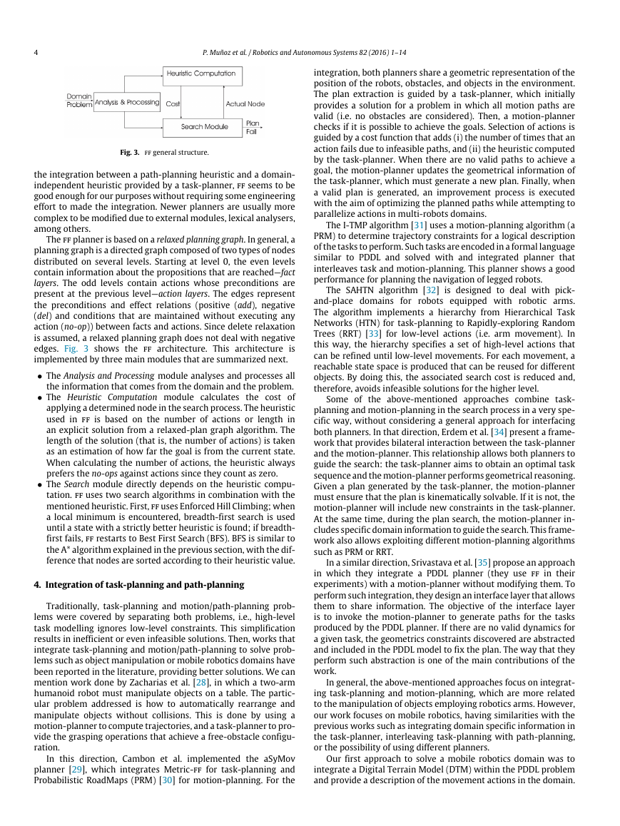
Fig. 4. Possible solutions to merge path-planning and task-planning.
Then, we solved the problem using a PDDL planner (see Fig. 4(a)).
However, this solution did not provide good results. The problem
of using a PDDL-based planner to integrate both path-planning and
task-planning presents two drawbacks. First, the complexity of the
domain and the problem. In our domain we used eight possible
movement actions north, south, east west, north-east, north-west,
south-east, and south-west. However, the critical part is in the
problem, where we need to provide the DTM in a grid form. This
means that we have to define all nodes and their connections. In
other words, what nodes are adjacent with each other. Second,
the size of the grids (at least 500 × 500 nodes). The planner must
instantiate a huge number of actions. Particularly, the movement
action is instantiated for every adjacent pair of nodes. Considering
the possibility of movement in eight directions, we can instantiate
eight possible move actions for each node. This results in an
exponential explosion of the search space. The more locations we
define in the problem, the more instantiated operators will be
generated. So, even for medium size maps, the search is intractable
and no state-of-the-art planner could solve it (partially or fully
grounded planners).
Solving small maps with this approach leads to routes with
headings restricted to multiples of π /4 since we have defined
movements in diagonal, horizontal and vertical, which may cause
sub-optimal paths. We could have defined more operators in order
to smooth this restriction, but the search was already intractable.
In this direction, we have first used ff, increasing the grid size.
Results show that the planner can manage 50 × 50 grids with 6
and 9 tasks in 1 and 2 s respectively, but requires a high amount
of memory (near 1 GB). Increasing the map size implies that ff is
unable to manage the problem size, and thus, it cannot provide a
solution. Since we wanted to test if the behaviour only occurred in
ff, we did the same test with other fully grounded planners such
as SGPlan, getting the same behaviour. We have also performed
the same test for the partially grounded planner SatPlan2006 [36].
Results were even less encouraging since more time was needed to
solve the basic problems that ff was able to solve.
A better solution is to decouple path-planning and task-
planning using a three phases planning process (see Fig. 4(b)). The
idea is to include a path-planner that generates a visibility graph
considering all the waypoints given in a PDDL problem (that is, the
initial and goal positions). This reduces the complexity of the PDDL
domain because all the movement actions are reduced to a single
one that traverses between waypoints. On the other hand, the
PDDL problem includes only the relevant positions. By doing this, it
is no longer required to include the DTM in the PDDL model, as the
path-planner considers it during the path-search. This reduction
in the number of actions and objects also decreases the workload
of the task-planner. Then, the PDDL planner provides a solution
in which there are movements between waypoints, but without
providing the real path between them. The last phase replaces the
movements between waypoints with a valid path by executing
again the path-planner. Finally, we obtain a plan in which tasks
and movements are properly interleaved.
This approach has two advantages (i) it allows to easily
interchange the PDDL planner and path-planner to exploit
different algorithms, and (ii) it eliminates zig-zag patterns and
provides better routes when it uses an any-angle path-planning
algorithm. However, this schema presents a major drawback: as
there is no shared information between the path-planner and the
task-planner during the search phase, solutions generated can be
highly inefficient. In particular, the election of the task-planner has
a big impact in the solution optimality as the domain independent
heuristic does not take into account the distance among task during
the search.
We have performed an experiment using SGPlan, OPTIC and
up2ta in a classical exploration domain where each task performs
a single action in a determined location. In particular, the test
consists of 10 maps of 100 × 100 nodes (considering a distance
between nodes of 1 m) with 20% of blocked cells. For each map, two
scenarios with 6 and 12 tasks randomly distributed are defined. For
all planners, the path-planning algorithm employed is S-Theta*,
so the differences in the path-length to accomplish all tasks are
due to the task ordering rather than the path-planning algorithm.
The average results of this test is shown in Table 1. Regardless of
the reduced number of scenarios tested, the difference between
the solutions provided is significant. SGPlan provides worse results
than OPTIC, but up2ta gives the best results. This is evidence that
when we merge the heuristic of the path-planner and the heuristic
of the task-planner we get better results than independently.
A detailed discussion on this issue will be presented in the
experimental sections.
5. Unified path-planning and task-planning architecture
The idea behind the up2ta planner comes from our experience
using a PDDL planner as the deliberative layer for the control of
a mobile robot in exploration domains. We wanted to develop
a planner that gets a closer to the optimal ordering of multiple
tasks placed in a grid. In order to do that, we combine a modified
ff planner and a path-planning algorithm to work together in
�
6
P. Muñoz et al. / Robotics and Autonomous Systems 82 (2016) 1–14
(a) Domain.
(b) Problem.
Fig. 5. Example PDDL files for the up2ta planner.
Table 1
Results for the execution of different problems with up2ta and two different PDDL-
based planners. In bold best values.
# tasks
6
12
Planner
SGplan
OPTIC
up2ta
SGPplan
OPTIC
up2ta
Runtime (ms)
2 007
2 653
1 661
8 364
69 800
8 917
Path length (m)
413.780
389.600
164.363
1785.121
1386.400
718.340
a coordinated way. The resulting system, called up2ta, takes
the benefits of (i) a PDDL planner for task-planning using PDDL
problems and domain independent heuristics, and (ii) a path-
planning algorithm for generating better routes using a DTM and
domain-specific heuristics.
The following subsections describe the files that are required by
the new planner and some concepts that we use later in this paper.
Then, we present the up2ta planner, with a special focus on how
the path-planning heuristic is combined with the heuristic search
planner.
5.1. Input files
The task-planner cannot have any path-planning related
operation. For this reason, the PDDL domain and problem do not
contain the DTM (this is only used by the path-planning algorithm).
The files required by up2ta are:
• Domain and problem: up2ta accepts any PDDL version that is
supported by the PDDL planner used in the integration. How-
ever, up2ta requires in the domain description an action called
Move_To that allows the robot to move between waypoints
(wp). Besides, the problem file does not need to provide a DTM,
just the waypoints in which we want to perform a task or tra-
verse through. These waypoints must have the form Ca_b to
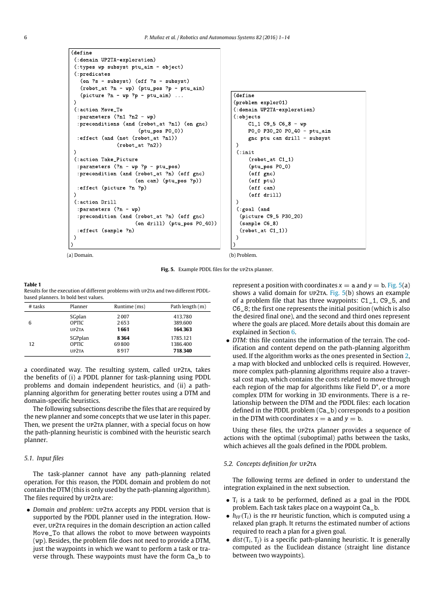
represent a position with coordinates x = a and y = b. Fig. 5(a)
shows a valid domain for up2ta. Fig. 5(b) shows an example
of a problem file that has three waypoints: C1_1, C9_5, and
C6_8; the first one represents the initial position (which is also
the desired final one), and the second and third ones represent
where the goals are placed. More details about this domain are
explained in Section 6.
• DTM: this file contains the information of the terrain. The cod-
ification and content depend on the path-planning algorithm
used. If the algorithm works as the ones presented in Section 2,
a map with blocked and unblocked cells is required. However,
more complex path-planning algorithms require also a traver-
sal cost map, which contains the costs related to move through
each region of the map for algorithms like Field D*, or a more
complex DTM for working in 3D environments. There is a re-
lationship between the DTM and the PDDL files: each location
defined in the PDDL problem (Ca_b) corresponds to a position
in the DTM with coordinates x = a and y = b.
Using these files, the up2ta planner provides a sequence of
actions with the optimal (suboptimal) paths between the tasks,
which achieves all the goals defined in the PDDL problem.
5.2. Concepts definition for up2ta
The following terms are defined in order to understand the
integration explained in the next subsection.
• Ti is a task to be performed, defined as a goal in the PDDL
problem. Each task takes place on a waypoint Ca_b.
• hFF (Ti) is the ff heuristic function, which is computed using a
relaxed plan graph. It returns the estimated number of actions
required to reach a plan for a given goal.
• dist(Ti, Tj) is a specific path-planning heuristic. It is generally
computed as the Euclidean distance (straight line distance
between two waypoints).
p�
P. Muñoz et al. / Robotics and Autonomous Systems 82 (2016) 1–14
7
finally the third goal T3 = robot_at C1_1. Note that the robot
ends at the same position where it starts.
As mentioned previously, the order in which we achieve the
goals has a significant impact in the quality solution due to the
total distance travelled. To optimally order the tasks, we have
modified the task-planner search algorithm to merge its heuristic
with the path-planner heuristic. For up2ta, we use ff as the task-
planner and S-Theta* as the path-planner algorithm. For the first
one, we have transformed the BFS algorithm into an A* algorithm.
The only difference between BFS and A* is that the latter includes
the heuristic computation in the node evaluation as is shown in
Eq. (1). In addition, we have disabled the Hill Climbing search to
avoid local minimums. For the path-planner, we do not need to
perform any modification. As we discuss later, the path-planner
algorithm is easy to replace with a different one.
Fig. 6. up2ta general structure.
• greedy(Ti, Tj) is the cost of a fast computed path between two
waypoints. This path is generated using a modified greedy path-
planning algorithm [13], which returns a suboptimal path with
lower runtime and memory usage.
• path(Ti, Tj) is the path length between two waypoints. This path
is computed using a classical path-planning algorithm such as.
A* or Theta*.
• H(Ti) is the heuristic function computed for a task. When a
task requires a movement between waypoints, the heuristic is
computed by adding the heuristic of the task-planner (hFF ) and
the heuristic from the path-planner.
• C(Ti) is the cost associated to perform Ti. This is value is
computed by the task-planner. Since we use ff, each action has
unit cost (for non-movement actions).
5.3. Integrated planner description
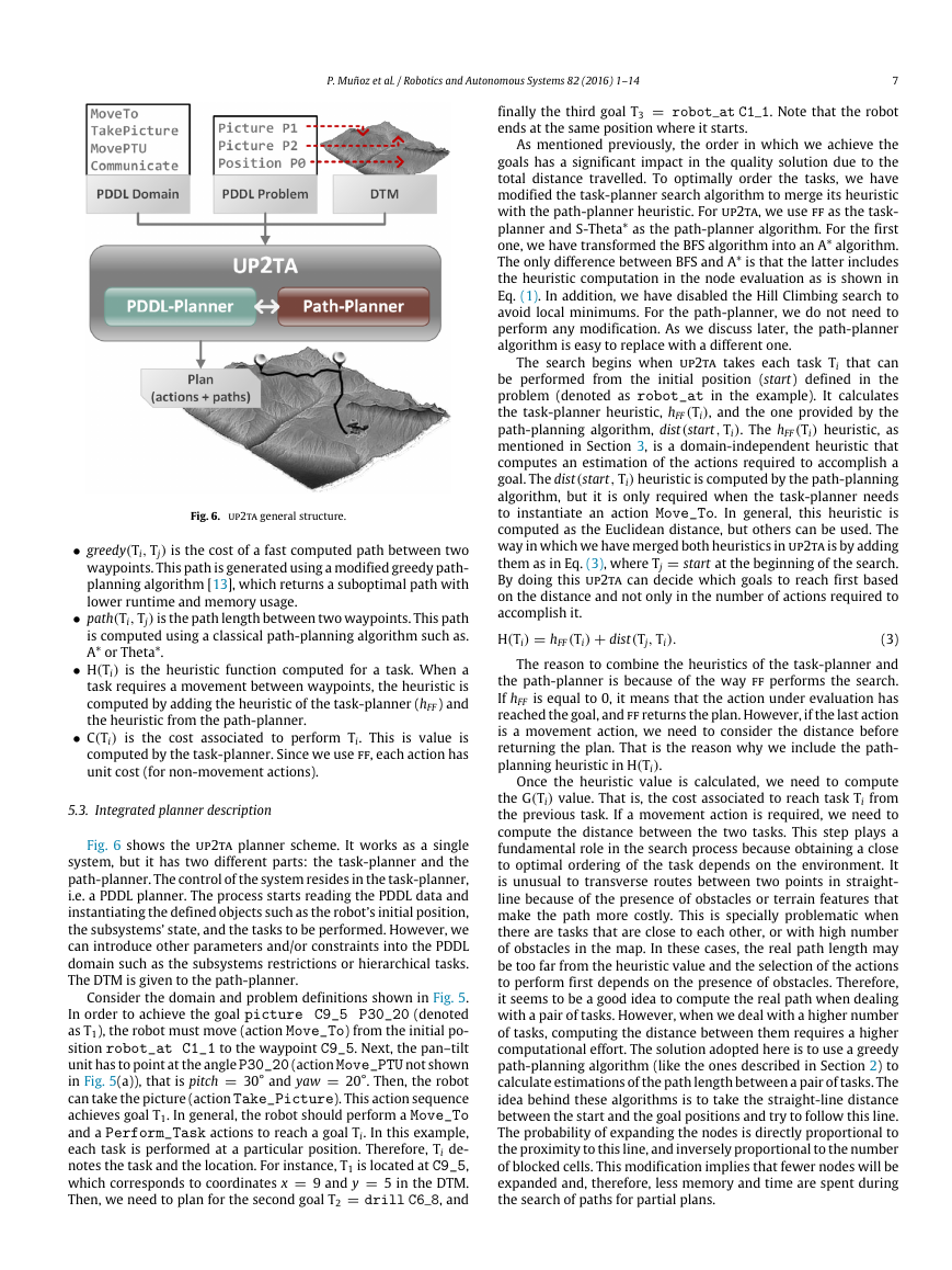
Fig. 6 shows the up2ta planner scheme. It works as a single
system, but it has two different parts: the task-planner and the
path-planner. The control of the system resides in the task-planner,
i.e. a PDDL planner. The process starts reading the PDDL data and
instantiating the defined objects such as the robot’s initial position,
the subsystems’ state, and the tasks to be performed. However, we
can introduce other parameters and/or constraints into the PDDL
domain such as the subsystems restrictions or hierarchical tasks.
The DTM is given to the path-planner.
Consider the domain and problem definitions shown in Fig. 5.
In order to achieve the goal picture C9_5 P30_20 (denoted
as T1), the robot must move (action Move_To) from the initial po-
sition robot_at C1_1 to the waypoint C9_5. Next, the pan–tilt
unit has to point at the angle P30_20 (action Move_PTU not shown
in Fig. 5(a)), that is pitch = 30° and yaw = 20°. Then, the robot
can take the picture (action Take_Picture). This action sequence
achieves goal T1. In general, the robot should perform a Move_To
and a Perform_Task actions to reach a goal Ti. In this example,
each task is performed at a particular position. Therefore, Ti de-
notes the task and the location. For instance, T1 is located at C9_5,
which corresponds to coordinates x = 9 and y = 5 in the DTM.
Then, we need to plan for the second goal T2 = drill C6_8, and
The search begins when up2ta takes each task Ti that can
be performed from the initial position (start) defined in the
problem (denoted as robot_at in the example). It calculates
the task-planner heuristic, hFF (Ti), and the one provided by the
path-planning algorithm, dist(start, Ti). The hFF (Ti) heuristic, as
mentioned in Section 3, is a domain-independent heuristic that
computes an estimation of the actions required to accomplish a
goal. The dist(start, Ti) heuristic is computed by the path-planning
algorithm, but it is only required when the task-planner needs
to instantiate an action Move_To. In general, this heuristic is
computed as the Euclidean distance, but others can be used. The
way in which we have merged both heuristics in up2ta is by adding
them as in Eq. (3), where Tj = start at the beginning of the search.
By doing this up2ta can decide which goals to reach first based
on the distance and not only in the number of actions required to
accomplish it.
H(Ti) = hFF (Ti) + dist(Tj, Ti).
(3)
The reason to combine the heuristics of the task-planner and
the path-planner is because of the way ff performs the search.
If hFF is equal to 0, it means that the action under evaluation has
reached the goal, and ff returns the plan. However, if the last action
is a movement action, we need to consider the distance before
returning the plan. That is the reason why we include the path-
planning heuristic in H(Ti).
Once the heuristic value is calculated, we need to compute
the G(Ti) value. That is, the cost associated to reach task Ti from
the previous task. If a movement action is required, we need to
compute the distance between the two tasks. This step plays a
fundamental role in the search process because obtaining a close
to optimal ordering of the task depends on the environment. It
is unusual to transverse routes between two points in straight-
line because of the presence of obstacles or terrain features that
make the path more costly. This is specially problematic when
there are tasks that are close to each other, or with high number
of obstacles in the map. In these cases, the real path length may
be too far from the heuristic value and the selection of the actions
to perform first depends on the presence of obstacles. Therefore,
it seems to be a good idea to compute the real path when dealing
with a pair of tasks. However, when we deal with a higher number
of tasks, computing the distance between them requires a higher
computational effort. The solution adopted here is to use a greedy
path-planning algorithm (like the ones described in Section 2) to
calculate estimations of the path length between a pair of tasks. The
idea behind these algorithms is to take the straight-line distance
between the start and the goal positions and try to follow this line.
The probability of expanding the nodes is directly proportional to
the proximity to this line, and inversely proportional to the number
of blocked cells. This modification implies that fewer nodes will be
expanded and, therefore, less memory and time are spent during
the search of paths for partial plans.
�
8
P. Muñoz et al. / Robotics and Autonomous Systems 82 (2016) 1–14
the heuristic given by the task-planner, i.e., the estimated number
of actions. The cost G(Ti) of achieving the position of each task is
calculated using Eq. (4). Once H(Ti) and G(Ti) are calculated, there
are three partial plans to be evaluated, one for each task Ti.
up2ta takes the one with lower F(Ti) value. In our example, it is
the partial plan that performs T1. Next, it evaluates the other two
possible tasks T2 and T3. In the same way, the system calculates the
heuristic and cost to reach T2 and T3 from T1, which in our case T2
has the lower value. At this point, there is only one remaining task
T3, so the search finishes by adding that task. Once all tasks have
been selected, the ordered tasks sequence for the solution is T1 →
T2 → T3. Fig. 8 shows the most promising partial plans connected
through a bold line (others have dotted lines). Then, up2ta will
calculate the real path between each pair of consecutive tasks
that have been previously ordered. Finally, the system provides an
ordered list of tasks and the paths between them.
6. Mobile robot exploration domains
In this section, we describe a scenario that we use in our
experimental evaluation. It consists of a mobile robot that must
achieve a set of exploration tasks in different locations. As
explained in Section 5.1, we must provide three files to up2ta: the
PDDL domain and problem, and the terrain information (DTM). The
PDDL domain was partially presented in Fig. 5. It describes robot
operations to manage the different subsystems (power on/off),
move between points (Move_To), and perform exploration tasks
(Take_Picture, Drill, etc.) to accomplish mission goals. The
robot is modelled to have different subsystems. In particular, it has
a scientific/navigation camera mounted on top of a pan–tilt unit,
a navigation subsystem, and drilling equipment. Each subsystem
can be on or off (must be on before operation). In addition, there
are some constraints that must be considered when operating
the different subsystems. Some of these constraints (shown in
Fig. 5(a)) are presented in the Move_To, Take_Picture, and
Drill acquisition operators. Concretely:
• In order to move between waypoints, the rover must power on
the navigation subsystem (gnc) and point the pan–tilt unit at
the front position (represented as P0_0) since the navigation
camera is mounted on it. The other subsystems must be off to
avoid mechanical problems and energy overconsumption.
• In order to take a picture, the rover must be stopped in the
desired location and with a specific pan–tilt position, which
are defined in the goal. The camera must be active and the
locomotion subsystem must be off.
• In order to get a sample from a desired location, the rover must
use the drilling equipment to perforate the subsurface. To do
this, the rover must be stopped in the desired position and the
pan–tilt unit must point at the surface—this allows the rover to
take pictures during the drilling process.
Initially, all rover’s subsystems are off with the pan–tilt unit
pointing to the front. The DTM, or terrain information, is in a
different file. Particularly, the one that we used within our path-
planning algorithms provides a grid with blocked and unblocked
cells (see Fig. 9(b)). Given these data, up2ta generates the solution
shown in Fig. 9(a). It is remarkable that the path-planner expands
the move actions between tasks to provide free collision paths,
while the task-planner orders the goals to minimize the distance
travelled for the final plan.
For this domain, each task can be performed independently.
That is, there is no relationship between tasks except for the robot
position. For this reason, we have also defined a more challenging
domain where tasks interfere with each other. This new domain is
an extension of the previous one that includes extra requirements
for the drilling process: it can only take one sample at a time,
Fig. 7. up2ta algorithm integration.
Although this approximation does not generate the real path,
the associated path length allows us to take into consideration the
presence of obstacles without spending a lot of time in obtaining
paths between tasks that probably will not be used in the final
solution. We define greedy(Ti, Tj) as the path cost between tasks
Ti and Tj using a greedy path-planning algorithm. In addition, we
need to compute the cost of the actions involved in performing
a task Ti. This value is represented as C(Ti) and it is given by the
task-planner. G(Ti) is a cumulative cost that depends on the cost of
reaching the previous task, the distance (estimated) between the
two tasks, and the cost of performing a task i as in Eq. (4) shows.
G(Ti) = greedy(Ti, Tj) + C(Ti) + G(Tj).
(4)
The task-planner keeps a list of partial plans (where a partial
plan is a plan that achieves an arbitrary task Ti) ordered by the
F(Ti) values. So, each time that the task-planner extracts a partial
plan, it adds it to the list. Then, the search process continues
with the extraction of the best promising partial plan. up2ta
generates all possible partial plans starting from the new location
where the robot is located. The task-planner continues extracting
partial plans until there are no more goals (all objectives are
accomplished), or there is no solution (unreachable task/s). When
all task are performed, up2ta does not give the solution directly.
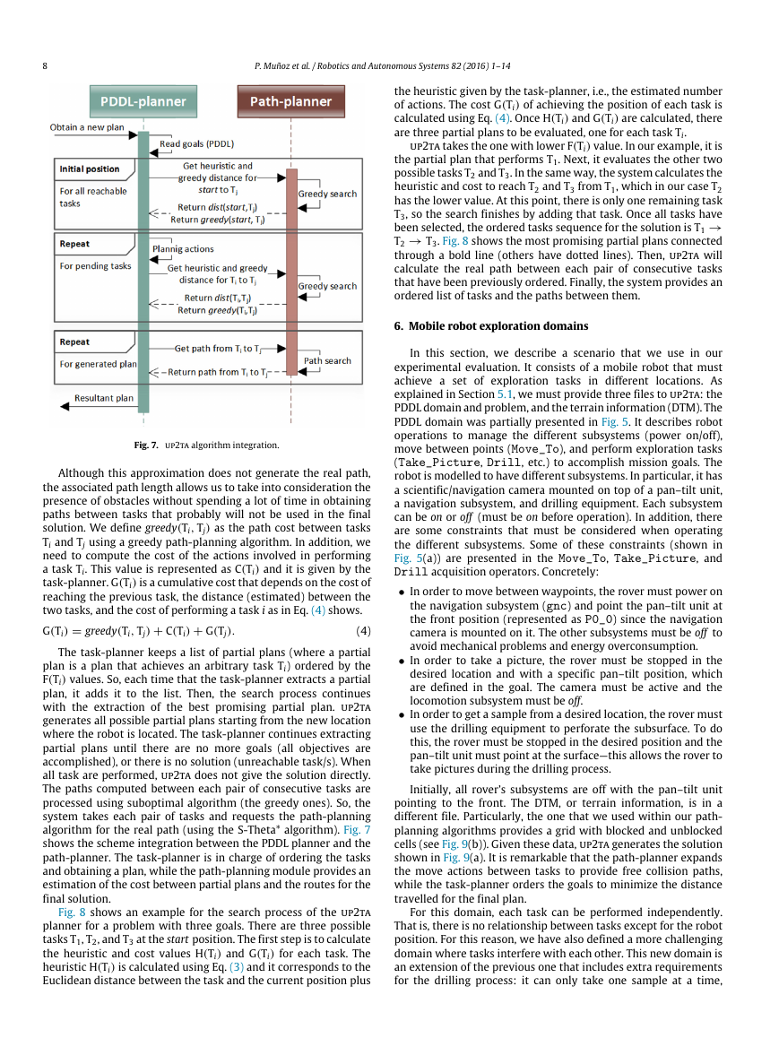
The paths computed between each pair of consecutive tasks are
processed using suboptimal algorithm (the greedy ones). So, the
system takes each pair of tasks and requests the path-planning
algorithm for the real path (using the S-Theta* algorithm). Fig. 7
shows the scheme integration between the PDDL planner and the
path-planner. The task-planner is in charge of ordering the tasks
and obtaining a plan, while the path-planning module provides an
estimation of the cost between partial plans and the routes for the
final solution.
Fig. 8 shows an example for the search process of the up2ta
planner for a problem with three goals. There are three possible
tasks T1, T2, and T3 at the start position. The first step is to calculate
the heuristic and cost values H(Ti) and G(Ti) for each task. The
heuristic H(Ti) is calculated using Eq. (3) and it corresponds to the
Euclidean distance between the task and the current position plus
�



 2023年江西萍乡中考道德与法治真题及答案.doc
 2012年重庆南川中考生物真题及答案.doc
 2013年江西师范大学地理学综合及文艺理论基础考研真题.doc
 2020年四川甘孜小升初语文真题及答案I卷.doc
 2020年注册岩土工程师专业基础考试真题及答案.doc
 2023-2024学年福建省厦门市九年级上学期数学月考试题及答案.doc
 2021-2022学年辽宁省沈阳市大东区九年级上学期语文期末试题及答案.doc
 2022-2023学年北京东城区初三第一学期物理期末试卷及答案.doc
 2018上半年江西教师资格初中地理学科知识与教学能力真题及答案.doc
 2012年河北国家公务员申论考试真题及答案-省级.doc
 2020-2021学年江苏省扬州市江都区邵樊片九年级上学期数学第一次质量检测试题及答案.doc
 2022下半年黑龙江教师资格证中学综合素质真题及答案.doc