This article has been accepted for publication in a future issue of this journal, but has not been fully edited. Content may change prior to final publication.
1
An Evolutionary Many-Objective Optimization
Algorithm Using Reference-point Based
Non-dominated Sorting Approach,
Part I: Solving Problems with Box Constraints
Kalyanmoy Deb, Fellow, IEEE and Himanshu Jain
Abstract—Having developed multi-objective optimization al-
gorithms using evolutionary optimization methods and demon-
strated their niche on various practical problems involving
mostly two and three objectives, there is now a growing need
for developing evolutionary multi-objective optimization (EMO)
algorithms for handling many-objective (having four or more
objectives) optimization problems. In this paper, we recognize a
few recent efforts and discuss a number of viable directions for
developing a potential EMO algorithm for solving many-objective
optimization problems. Thereafter, we suggest a reference-point
based many-objective NSGA-II (we call it NSGA-III) that em-
phasizes population members which are non-dominated yet close
to a set of supplied reference points. The proposed NSGA-III is
applied to a number of many-objective test problems having two
to 15 objectives and compared with two versions of a recently
suggested EMO algorithm (MOEA/D). While each of the two
MOEA/D methods works well on different classes of problems,
the proposed NSGA-III is found to produce satisfactory results
on all problems considered in this study. This paper presents
results on unconstrained problems and the sequel paper considers
constrained and other specialties in handling many-objective
optimization problems.
Index Terms—Many-objective optimization, evolutionary com-
large dimension, NSGA-III, non-dominated sorting,
putation,
multi-criterion optimization.
I. INTRODUCTION
Evolutionary multi-objective optimization (EMO) method-
ologies have amply shown their niche in finding a set of
well-converged and well-diversified non-dominated solutions
in different two and three-objective optimization problems
since the beginning of nineties. However, in most real-world
problems involving multiple stake-holders and functionalities,
there often exists many optimization problems that involve
four or more objectives, sometimes demanding to have 10 to
15 objectives [1], [2]. Thus, it is not surprising that handling a
large number of objectives had been one of the main research
activities in EMO for the past few years. Many-objective
K. Deb is with Department of Electrical and Computer Engineering.
Michigan State University, 428 S. Shaw Lane, 2120 EB, East Lansing, MI
48824, USA, e-mail: kdeb@egr.msu.edu (see http://www.egr.msu.edu/˜kdeb).
Prof. Deb is also a visiting professor at Aalto University School of Business,
Finland and University of Sk¨ovde, Sweden.
H. Jain is with Eaton Corporation, Pune 411014, India, email: himan-
shu.j689@gmail.com.
Copyright (c) 2012 IEEE. Personal use of this material
is permitted.
However, permission to use this material for any other purposes must be
obtained from the IEEE by sending a request to pubs-permissions@ieee.org.
problems pose a number of challenges to any optimization
algorithm, including an EMO. First and foremost, the propor-
tion of non-dominated solutions in a randomly chosen set of
objective vectors becomes exponentially large with an increase
of number of objectives. Since the non-dominated solutions
occupy most of the population slots, any elite-preserving
EMO faces a difficulty in accommodating adequate number
of new solutions in the population. This slows down the
search process considerably [3], [4]. Second, implementation
of a diversity-preservation operator (such as the crowding
distance operator [5] or clustering operator [6]) becomes a
computationally expensive operation. Third, visualization of
a large-dimensional front becomes a difficult task, thereby
causing difficulties in subsequent decision-making tasks and in
evaluating the performance of an algorithm. For this purpose,
the performance metrics (such as hyper-volume measure [7] or
other metrics [3], [8]) are either computationally too expensive
or may not be meaningful.
An important question to ask is then ‘Are EMOs useful for
many-objective optimization problems?’. Although the third
difficulty related to visualization and performance measures
mentioned above cannot be avoided, some algorithmic changes
to the existing EMO algorithms may be possible to address
the first
two concerns. In this paper, we review some of
the past efforts [9], [10], [11], [12], [13], [14] in devising
many-objective EMOs and outline some viable directions
for designing efficient many-objective EMO methodologies.
Thereafter, we propose a new method that uses the framework
of NSGA-II procedure [5] but works with a set of supplied
or predefined reference points and demonstrate its efficacy in
solving two to 15-objective optimization problems. In this
paper, we introduce the framework and restrict to solving
unconstrained problems of various kinds, such as having
normalized, scaled, convex, concave, disjointed, and focusing
on a part of the Pareto-optimal front. Practice may offer a
number of such properties to exist in a problem. Therefore, an
adequate test of an algorithm for these eventualities remains
as an important task. We compare the performance of the
proposed NSGA-III with two versions of an existing many-
objective EMO (MOEA/D [10]), as the method is somewhat
similar to the proposed method. Interesting insights about
working of both versions of MOEA/D and NSGA-III are
revealed. The proposed NSGA-III is also evaluated for its
use in a few other interesting multi-objective optimization and
Copyright (c) 2013 IEEE. Personal use is permitted. For any other purposes, permission must be obtained from the IEEE by emailing pubs-permissions@ieee.org.
�
This article has been accepted for publication in a future issue of this journal, but has not been fully edited. Content may change prior to final publication.
decision-making tasks. In the sequel of this paper, we suggest
an extension of the proposed NSGA-III for handling many-
objective constrained optimization problems and a few other
special and challenging many-objective problems.
In the remainder of this paper, we first discuss the diffi-
culties in solving many-objective optimization problems and
then attempt to answer the question posed above about the
usefulness of EMO algorithms in handling many objectives.
Thereafter, in Section III, we present a review of some of
the past studies on many-objective optimization including a
recently proposed method MOEA/D [10]. Then, in Section IV,
we outline our proposed NSGA-III procedure in detail. Results
on normalized DTLZ test problems up to 15 objectives using
NSGA-III and two versions of MOEA/D are presented next
in Section V-A. Results on scaled version of DTLZ problems
suggested here are shown next. Thereafter in subsequent
sections, NSGA-III procedure is tested on different
types
of many-objective optimization problems. Finally, NSGA-III
is applied to two practical problems involving three and
nine objective problems in Section VII. Conclusions of this
extensive study are drawn in Section VIII.
II. MANY-OBJECTIVE PROBLEMS
Loosely, many-objective problems are defined as problems
having four or more objectives. Two and three-objective prob-
lems fall into a different class as the resulting Pareto-optimal
front, in most cases, in its totality can be comprehensively
visualized using graphical means. Although a strict upper
bound on the number of objectives for a many-objective
optimization problem is not so clear, except a few occasions
[15], most practitioners are interested in a maximum of 10
to 15 objectives. In this section, first, we discuss difficulties
that an existing EMO algorithm may face in handling many-
objective problems and investigate if EMO algorithms are
useful at all in handling a large number of objectives.
2
may cause an unacceptable distribution of solutions at
the end.
3) Recombination operation may be inefficient: In a many-
objective problem, if only a handful of solutions are
to be found in a large-dimensional space, solutions are
likely to be widely distant from each other. In such a
population, the effect of recombination operator (which
is considered as a key search operator in an EMO)
becomes questionable. Two distant parent solutions are
likely to produce offspring solutions that are also distant
from parents. Thus, special recombination operators
(mating restriction or other schemes) may be necessary
for handling many-objective problems efficiently.
4) Representation of
trade-off surface is difficult: It
is
intuitive to realize that to represent a higher dimensional
trade-off surface, exponentially more points are needed.
Thus, a large population size is needed to represent the
resulting Pareto-optimal front. This causes difficulty for
a decision-maker to comprehend and make an adequate
decision to choose a preferred solution.
5) Performance metrics are computationally expensive to
compute: Since higher-dimensional sets of points are
to be compared against each other to establish the
performance of one algorithm against another, a larger
computational effort is needed. For example, computing
hyper-volume metric requires exponentially more com-
putations with the number of objectives [18], [19].
6) Visualization is difficult: Finally, although it is not a
matter related to optimization directly, eventually visu-
alization of a higher-dimensional trade-off front may be
difficult for many-objective problems.
The first three difficulties can only be alleviated by certain
modifications to existing EMO methodologies. The fourth,
fifth, and sixth difficulties are common to all many-objective
optimization problems and we do not address them adequately
here.
A. Difficulties in Handling Many Objectives
It has been discussed elsewhere [4], [16] that the current
state-of-the-art EMO algorithms that work under the principle
of domination [17] may face the following difficulties:
1) A large fraction of population is non-dominated: It is
well-known [3], [16] that with an increase in number
of objectives, an increasingly larger fraction of a ran-
domly generated population becomes non-dominated.
Since most EMO algorithms emphasize non-dominated
solutions in a population, in handling many-objective
problems, there is not much room for creating new
solutions in a generation. This slows down the search
process and therefore the overall EMO algorithm be-
comes inefficient.
2) Evaluation of diversity measure becomes computation-
ally expensive: To determine the extent of crowding of
solutions in a population, the identification of neigh-
bors becomes computationally expensive in a large-
dimensional space. Any compromise or approximation
in diversity estimate to make the computations faster
B. EMO Methodologies for Handling Many-Objective Prob-
lems
Before we discuss the possible remedies for three difficulties
mentioned above, here we highlight
two different many-
objective problem classes for which existing EMO method-
ologies can still be used.
First, existing EMO algorithms may still be useful in finding
a preferred subset of solutions (a partial set) from the complete
Pareto-optimal set. Although the preferred subset will still be
many-dimensional, since the targeted solutions are focused in
a small region on the Pareto-optimal front, most of the above
difficulties will be alleviated by this principle. A number of
MCDM-based EMO methodologies are already devised for
this purpose and results on as large as 10-objective problems
have shown to perform well [20], [21], [22], [23].
Second, many problems in practice, albeit having many
objectives, often degenerate to result in a low-dimensional
Pareto-optimal front [4], [11], [24], [25]. In such problems,
identification of redundant objectives can be integrated with an
EMO to find the Pareto-optimal front that is low-dimensional.
Copyright (c) 2013 IEEE. Personal use is permitted. For any other purposes, permission must be obtained from the IEEE by emailing pubs-permissions@ieee.org.
�
This article has been accepted for publication in a future issue of this journal, but has not been fully edited. Content may change prior to final publication.
Since the ultimate front is as low as two or three-dimensional,
existing EMO methodologies should work well in handling
such problems. A previous study of NSGA-II with a principal
component analysis (PCA) based procedure [4] was able to
solve as large as 50-objective problems having a two-objective
Pareto-optimal front.
C. Two Ideas for a Many-Objective EMO
Keeping in mind the first three difficulties associated with
a domination-based EMO procedure, two different strategies
can be considered to alleviate the difficulties:
1) Use of a special domination principle: The first difficulty
mentioned above can be alleviated by using a special
domination principle that will adaptively discretize the
Pareto-optimal front and find a well-distributed set of
points. For example, the use of �-domination principle
[26], [27] will make all points within � distance from a
set of Pareto-optimal points �-dominated and hence the
process will generate a finite number of Pareto-optimal
points as target. Such a consideration will also alleviate
the second difficulty of diversity preservation. The third
difficulty can be taken care of by the use of a mating
restriction scheme or a special recombination scheme
in which near-parent solutions are emphasized (such as
SBX with a large distribution index [28]). Other special
domination principles [29], [30] can also be used for this
purpose. Aguirre and Tanaka [31] and Sato et al. [32]
suggested the use of a subset of objectives for dominance
check and using a different combination of objectives in
every generation. The use of fixed cone-domination [33],
[34] or variable cone-domination [35] principles can also
be tried. These studies were made in the context of low-
dimensional problems and their success in solving many-
objective optimization is yet to be established.
2) Use of a predefined multiple targeted search: It has
been increasingly clear that it is too much to expect
from a single population-based optimization algorithm
to have convergence of its population near the Pareto-
optimal front and simultaneously its distributed uni-
formly around the entire front in a large-dimensional
problem. One way to handle such many-objective opti-
mization problems would be to aid the diversity mainte-
nance issue by some external means. This principle can
directly address the second difficulty mentioned above.
Instead of searching the entire search space for Pareto-
optimal solutions, multiple predefined targeted searches
can be set by an algorithm. Since optimal points are
found corresponding to each of the targeted search task,
the first difficulty of dealing with a large non-dominated
set is also alleviated. The recombination issue can be
addressed by using a mating restriction scheme in which
two solutions from neighboring targets are participated
in the recombination operation. Our proposed algorithm
(NSGA-III) is based on this principle and thus we
discuss this aspect in somewhat more detail. We suggest
two different ways to implement the predefined multiple
targeted search principle:
3
a) A set of predefined search directions spanning
the entire Pareto-optimal front can be specified
beforehand and multiple searches can be performed
along each direction. Since the search directions
are widely distributed, the obtained optimal points
are also likely to be widely distributed on the
Pareto-optimal front in most problems. Recently
proposed MOEA/D procedure [10] uses this con-
cept.
b) Instead of multiple search directions, multiple pre-
defined reference points can be specified for this
purpose. Thereafter, points corresponding to each
reference point can be emphasized to find set of
widely distributed set of Pareto-optimal points. A
few such implementations were proposed recently
[36], [37], [38], [14], and this paper suggests
another approach extending and perfecting the al-
gorithm proposed in the first reference [36].
III. EXISTING MANY-OBJECTIVE OPTIMIZATION
ALGORITHMS
Garza-Fabre, Pulido and Coello [16] suggested three single-
objective measures by using differences in individual objective
values between two competing parents and showed that in 5 to
50-objective DTLZ1, DTLZ3 and DTLZ6 problems the con-
vergence property can get enhanced compared to a number of
existing methods including the usual Pareto-dominance based
EMO approaches. Purshouse and Fleming [39] clearly showed
that diversity preservation and achieving convergence near the
Pareto-optimal front are two contradictory goals and usual
genetic operators are not adequate to attain both goals simul-
taneously, particularly for many-objective problems. Another
study [40] extends NSGA-II by adding diversity-controlling
operators to solve six to 20-objective DTLZ2 problems.
K¨oppen and Yoshida [41] claimed that NSGA-II procedure
in its originality is not suitable for many-objective optimiza-
tion problems and suggested a number of metrics that can
potentially replace NSGA-II’s crowding distance operator for
better performance. Based on simulation studies on two to
15-objective DTLZ2, DTLZ3 and DTLZ6 problems,
they
suggested to use a substitute assignment distance measure as
the best strategy. Hadka and Reed [42] suggested an ensemble-
based EMO procedure which uses a suitable recombination
operator adaptively chosen from a set of eight to 10 different
pre-defined operators based on their generation-wise success
rate in a problem. It also uses �-dominance concept and an
adaptive population sizing approach that is reported to solve
up to eight-objective test problems successfully. Bader and
Zitzler [43] have suggested a fast procedure for computing
sample-based hyper-volume and devised an algorithm to find a
set of trade-off solutions for maximizing the hyper-volume. A
growing literature on approximate hyper-volume computation
[44], [18], [45] may make such an approach practical for
solving many-objective problems.
The above studies analyze and extend previously-suggested
evolutionary multi-objective optimization algorithms for their
suitability to solving many-objective problems. In most cases,
Copyright (c) 2013 IEEE. Personal use is permitted. For any other purposes, permission must be obtained from the IEEE by emailing pubs-permissions@ieee.org.
�
This article has been accepted for publication in a future issue of this journal, but has not been fully edited. Content may change prior to final publication.
the results are promising and the suggested algorithms must
be tested on other more challenging problems than the usual
normalized test problems such as DTLZ problems. They
must also be tried on real-world problems. In the following
paragraphs, we describe a recently proposed algorithm which
fits well with our description of a many-objective optimization
algorithm given in Section II-C and closely matches with our
proposed algorithm.
MOEA/D [10] uses a predefined set of weight vectors to
maintain a diverse set of trade-off solutions. For each weight
vector, the resulting problem is called a sub-problem. To start
with, every population member (with size same as the number
of weight vectors) is associated with a weight vector randomly.
Thereafter, two solutions from neighboring weight vectors
(defined through a niching parameter (T )) are mated and an
offspring solution is created. The offspring is then associated
with one or more weight vectors based on a performance
metric. Two metrics are suggested in the study. A penalized
distance measure of a point from the ideal point is formed by
weighted sum (weight θ is another algorithmic parameter) of
perpendicular distance (d2) from the reference direction and
distance (d1) along the reference direction:
PBI(x, w) = d1 + θd2.
(1)
We call this procedure here as MOEA/D-PBI. The second
approach suggested is the use of Tchebycheff metric using
a utopian point z∗ and the weight vector w:
TCH(x, w, z∗) =
M
max
i=1
wi|fi(x) − z∗
i |.
(2)
In reported simulations [10], the ideal point was used as z∗
and zero-weight scenario is handled by using a small number.
We call this procedure as MOEA/D-TCH here. An external
population maintains the non-dominated solutions. The first
two difficulties mentioned earlier are negotiated by using an
explicit set of weight vectors to find points and the third
difficulty is alleviated by using a mating restriction scheme.
Simulation results were shown for two and three-objective test
problems only and it was concluded that MOEA/D-PBI is
better for three-objective problems than MOEA/D-TCH and
the performance of MOEA/D-TCH improved with an objective
normalization process using population minimum and maxi-
mum objective values. Both versions of MOEA/D require to
set a niching parameter (T ). Based on some simulation results
on two and three-objective problems, authors suggested the
use of a large fraction of population size as T . Additionally,
MOEA/D-PBI requires an appropriate setting of an additional
parameter – penalty parameter θ, for which authors have
suggested a value of 5.
A later study by the developers of MOEA/D suggested
the use of differential evolution (DE) to replace genetic
recombination and mutation operators. Also, further modifi-
cations were done in defining neighborhood of a particular
solution and in replacing parents in a given neighborhood
by the corresponding offspring solutions [46]. We call this
method as MOEA/D-DE here. Results on a set of mostly
two and a three-objective linked problems [47] showed better
performance with MOEA/D-DE compared to other algorithms.
4
As mentioned, MOEA/D is a promising approach for many-
objective optimization as it addresses some of the difficulties
mentioned above well, but the above-mentioned MOEA/D
studies did not quite explore their suitability to a large number
of objectives. In this paper, we apply them to problems having
up to 15 objectives and evaluate their applicability to truly
many-objective optimization problems and reveal interesting
properties of these algorithms.
Another recent study [14] follows our description of a
many-objective optimization procedure. The study extends
the NSGA-II procedure to suggest a hybrid NSGA-II (HN
algorithm) for handling three and four-objective problems.
Combined population members are projected on a hyper-
plane and a clustering operation is performed on the hyper-
plane to select a desired number of clusters which is user-
defined. Thereafter, based on the diversity of the population,
either a local search operation on a random cluster member
is used to move the solution closer to the Pareto-optimal
front or a diversity enhancement operator is used to choose
population members from all clusters. Since no targeted and
distributed search is used, the approach is more generic than
MOEA/D or the procedure suggested in this paper. However,
the efficiency of HN algorithm for problems having more than
four objectives is yet to be investigated to suggest its use for
many-objective problems, in general. We now describe our
proposed algorithm.
IV. PROPOSED ALGORITHM: NSGA-III
(or NSGA-III)
remains similar
The basic framework of
the proposed many-objective
NSGA-II
to the original
NSGA-II algorithm [5] with significant changes in its selec-
tion mechanism. But unlike in NSGA-II, the maintenance of
diversity among population members in NSGA-III is aided by
supplying and adaptively updating a number of well-spread
reference points. For completeness, we first present a brief
description of the original NSGA-II algorithm.
Let us consider t-th generation of NSGA-II algorithm.
Suppose the parent population at this generation is Pt and
its size is N , while the offspring population created from Pt
is Qt having N members. The first step is to choose the
best N members from the combined parent and offspring
population Rt = Pt ∪ Qt (of size 2N ), thus allowing to
preserve elite members of the parent population. To achieve
this, first, the combined population Rt is sorted according to
different non-domination levels (F1, F2 and so on). Then, each
non-domination level is selected one at a time to construct a
new population St, starting from F1, until the size of St is
equal to N or for the first time exceeds N . Let us say the last
level included is the l-th level. Thus, all solutions from level
(l + 1) onwards are rejected from the combined population
Rt. In most situations, the last accepted level (l-th level) is
only accepted partially. In such a case, only those solutions
that will maximize the diversity of the l-th front are chosen. In
NSGA-II, this is achieved through a computationally efficient
yet approximate niche-preservation operator which computes
the crowding distance for every last level member as the
summation of objective-wise normalized distance between two
Copyright (c) 2013 IEEE. Personal use is permitted. For any other purposes, permission must be obtained from the IEEE by emailing pubs-permissions@ieee.org.
�
This article has been accepted for publication in a future issue of this journal, but has not been fully edited. Content may change prior to final publication.
5
neighboring solutions. Thereafter, the solutions having larger
crowding distance values are chosen. Here, we replace the
crowding distance operator with the following approaches
(subsections IV-A to IV-E).
A. Classification of Population into Non-dominated Levels
The above procedure of identifying non-dominated fronts
using the usual domination principle [17] is also used in
NSGA-III. All population members from non-dominated front
level 1 to level l are first included in St. If |St| = N , no further
operations are needed and the next generation is started with
Pt+1 = St. For |St| > N , members from one to (l − 1)
fronts are already selected, that is, Pt+1 = ∪l−1
i=1Fi, and the
remaining (K = N −| Pt+1|) population members are chosen
from the last front Fl. We describe the remaining selection
process in the following subsections.
B. Determination of Reference Points on a Hyper-Plane
As indicated before, NSGA-III uses a predefined set of
reference points to ensure diversity in obtained solutions.
The chosen reference points can either be predefined in a
structured manner or supplied preferentially by the user. We
shall present results of both methods in the results section later.
In the absence of any preference information, any predefined
structured placement of reference points can be adopted, but in
this paper we use Das and Dennis’s [48] systematic approach1
that places points on a normalized hyper-plane – a (M − 1)-
dimensional unit simplex – which is equally inclined to all
objective axes and has an intercept of one on each axis. If p
divisions are considered along each objective, the total number
of reference points (H) in an M -objective problem is given
by:
H = !M + p − 1
p
".
(3)
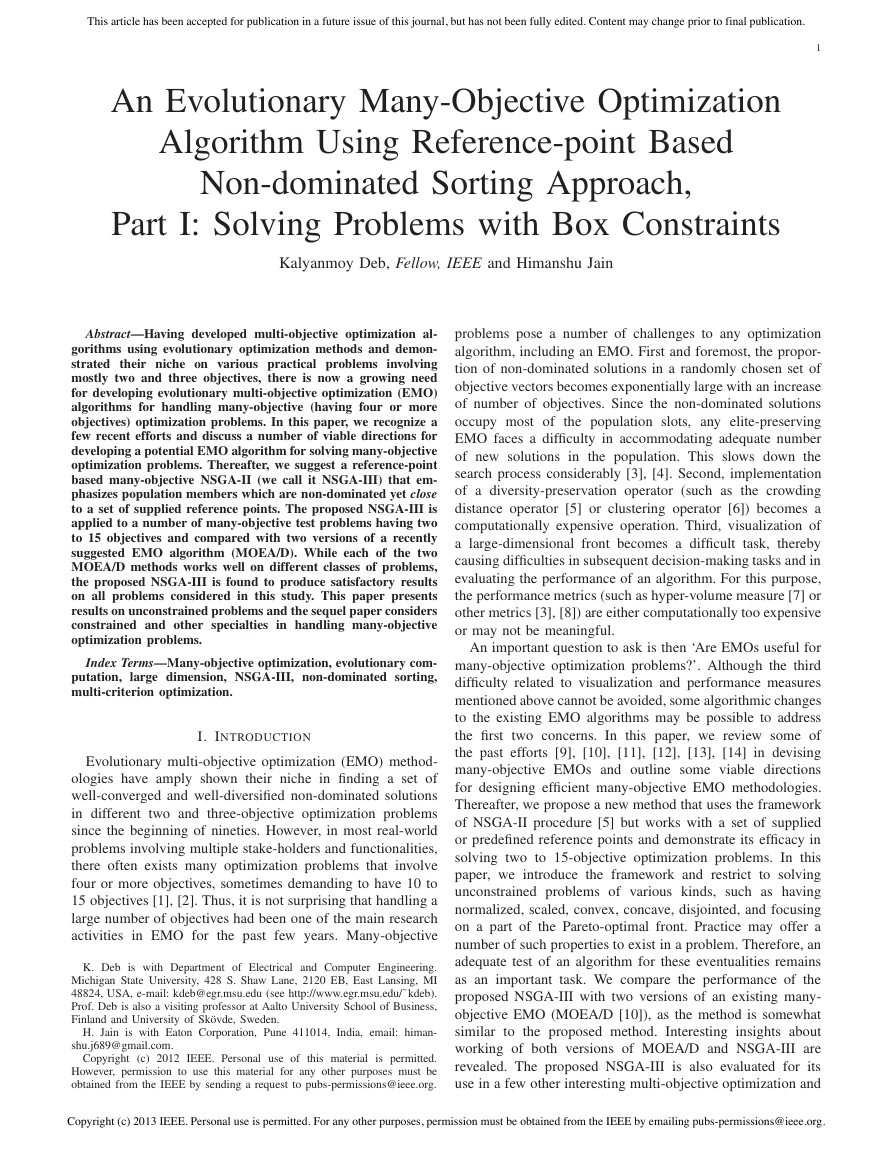
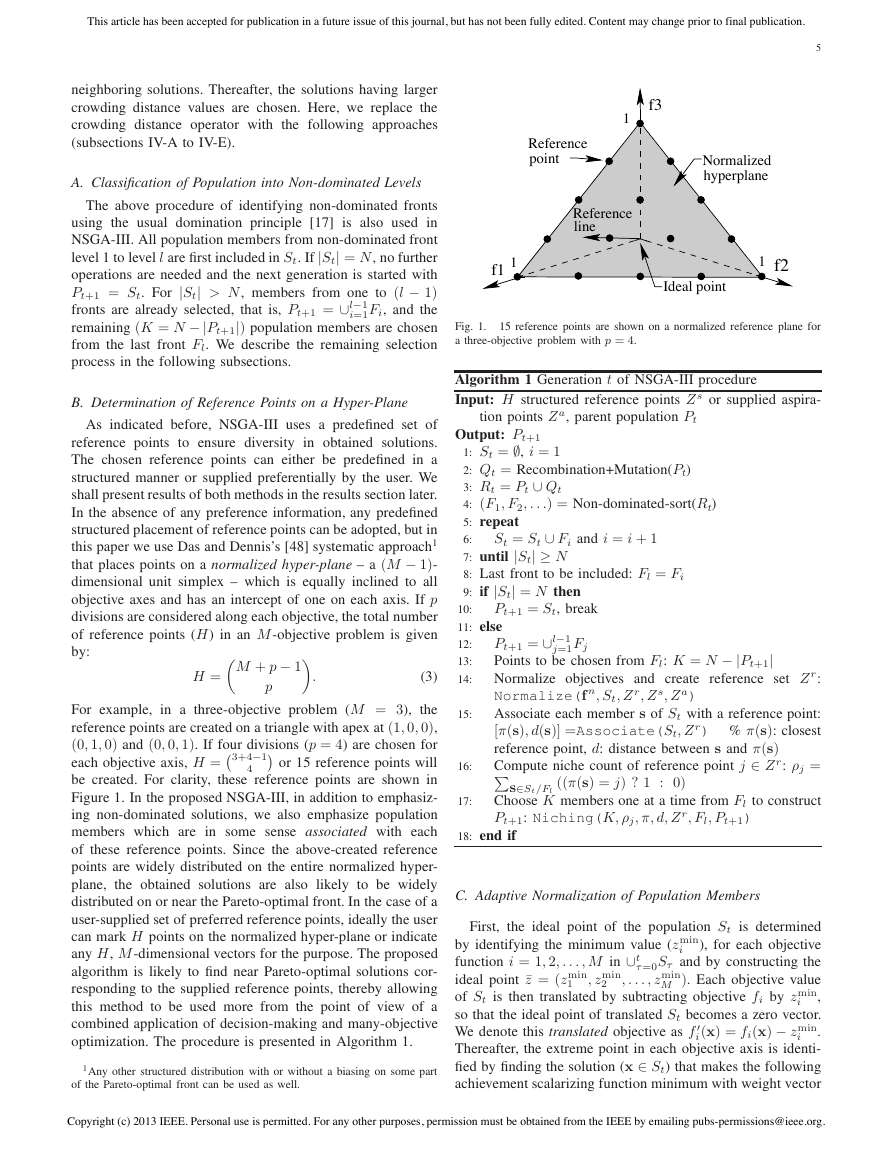
For example, in a three-objective problem (M = 3), the
reference points are created on a triangle with apex at (1, 0, 0),
(0, 1, 0) and (0, 0, 1). If four divisions (p = 4) are chosen for
each objective axis, H = #3+4−1
4
$ or 15 reference points will
be created. For clarity, these reference points are shown in
Figure 1. In the proposed NSGA-III, in addition to emphasiz-
ing non-dominated solutions, we also emphasize population
members which are in some sense associated with each
of these reference points. Since the above-created reference
points are widely distributed on the entire normalized hyper-
plane, the obtained solutions are also likely to be widely
distributed on or near the Pareto-optimal front. In the case of a
user-supplied set of preferred reference points, ideally the user
can mark H points on the normalized hyper-plane or indicate
any H, M -dimensional vectors for the purpose. The proposed
algorithm is likely to find near Pareto-optimal solutions cor-
responding to the supplied reference points, thereby allowing
this method to be used more from the point of view of a
combined application of decision-making and many-objective
optimization. The procedure is presented in Algorithm 1.
1Any other structured distribution with or without a biasing on some part
of the Pareto-optimal front can be used as well.
f3
1
Reference
point
Reference
line
Normalized
hyperplane
1f1
1 f2
Ideal point
Fig. 1.
a three-objective problem with p = 4.
15 reference points are shown on a normalized reference plane for
Algorithm 1 Generation t of NSGA-III procedure
Input: H structured reference points Z s or supplied aspira-
tion points Z a, parent population Pt
Output: Pt+1
St = St ∪ Fi and i = i + 1
1: St = ∅, i = 1
2: Qt = Recombination+Mutation(Pt)
3: Rt = Pt ∪ Qt
4: (F1, F2, . . .) = Non-dominated-sort(Rt)
5: repeat
6:
7: until |St|≥ N
8: Last front to be included: Fl = Fi
9: if |St| = N then
10:
11: else
12:
Pt+1 = St, break
13:
14:
15:
16:
17:
j=1Fj
Pt+1 = ∪l−1
Points to be chosen from Fl: K = N −| Pt+1|
Normalize objectives and create reference set Z r:
Normalize(f n, St, Z r, Z s, Z a)
Associate each member s of St with a reference point:
[π(s), d(s)] =Associate(St, Z r) % π(s): closest
reference point, d: distance between s and π(s)
Compute niche count of reference point j ∈ Z r: ρj =
%s∈St/Fl
Choose K members one at a time from Fl to construct
Pt+1: Niching(K, ρj,π, d, Z r, Fl, Pt+1)
((π(s) = j) ? 1 : 0)
18: end if
C. Adaptive Normalization of Population Members
i
1
, zmin
First, the ideal point of the population St is determined
by identifying the minimum value (zmin
), for each objective
function i = 1, 2, . . . , M in ∪t
τ =0Sτ and by constructing the
ideal point ¯z = (zmin
M ). Each objective value
of St is then translated by subtracting objective fi by zmin
,
so that the ideal point of translated St becomes a zero vector.
We denote this translated objective as f $
i(x) = fi(x) − zmin
.
Thereafter, the extreme point in each objective axis is identi-
fied by finding the solution (x ∈ St) that makes the following
achievement scalarizing function minimum with weight vector
, . . . , zmin
2
i
i
Copyright (c) 2013 IEEE. Personal use is permitted. For any other purposes, permission must be obtained from the IEEE by emailing pubs-permissions@ieee.org.
�
This article has been accepted for publication in a future issue of this journal, but has not been fully edited. Content may change prior to final publication.
6
w being the axis direction:
ASF (x, w) =
M
max
i=1
f $
i(x)/wi,
for x ∈ St.
(4)
For wi = 0, we replace it with a small number 10−6. For i-th
translated objective direction f $
i , this will result in an extreme
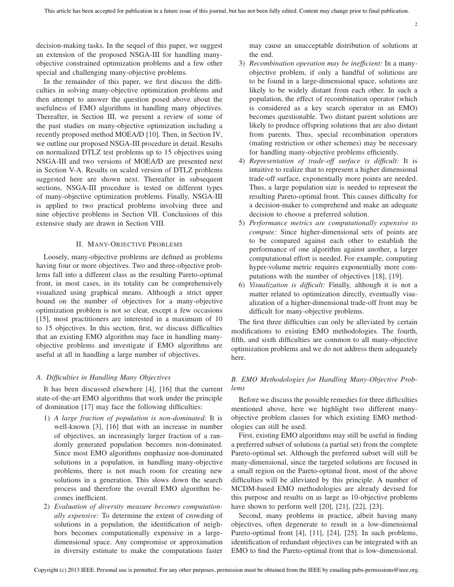
objective vector, zi,max. These M extreme vectors are then
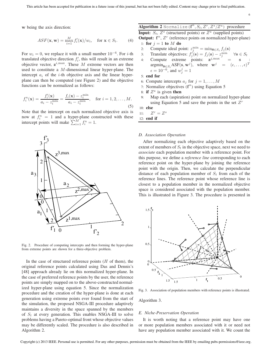
used to constitute a M -dimensional linear hyper-plane. The
intercept ai of the i-th objective axis and the linear hyper-
plane can then be computed (see Figure 2) and the objective
functions can be normalized as follows:
f n
i (x) =
f $
i(x)
ai − zmin
i
=
fi(x) − zmin
i
ai − zmin
i
,
for i = 1, 2, . . . , M .
(5)
Note that the intercept on each normalized objective axis is
now at f n
i = 1 and a hyper-plane constructed with these
intercept points will make %M
i=1 f n
i = 1.
3a
f’
3
3
2
1
0
0
a1
1
3,max
z
2a
2,max
z
1,max
z
2
f’
1
0
1
f’
2
2
Fig. 2. Procedure of computing intercepts and then forming the hyper-plane
from extreme points are shown for a three-objective problem.
In the case of structured reference points (H of them), the
original reference points calculated using Das and Dennis’s
[48] approach already lie on this normalized hyper-plane. In
the case of preferred reference points by the user, the reference
points are simply mapped on to the above-constructed normal-
ized hyper-plane using equation 5. Since the normalization
procedure and the creation of the hyper-plane is done at each
generation using extreme points ever found from the start of
the simulation, the proposed NSGA-III procedure adaptively
maintains a diversity in the space spanned by the members
of St at every generation. This enables NSGA-III to solve
problems having a Pareto-optimal front whose objective values
may be differently scaled. The procedure is also described in
Algorithm 2.
Algorithm 2 Normalize(f n, St, Z r, Z s/Z a) procedure
Input: St, Z s (structured points) or Z a (supplied points)
Output: f n, Z r (reference points on normalized hyper-plane)
1: for j = 1 to M do
2:
3:
4:
Compute ideal point: zmin
Translate objectives: f $
Compute
argmins∈St
� = 10−6, and wj
j = 1
j = mins∈St fj(s)
j(s) = fj(s) − zmin
points:
zj,max
j
∀s ∈ St
:
extreme
ASF(s, wj), where wj = (�, . . . , �)T
=
s
5: end for
6: Compute intercepts aj for j = 1, . . . , M
7: Normalize objectives (f n) using Equation 5
8: if Z a is given then
9: Map each (aspiration) point on normalized hyper-plane
using Equation 5 and save the points in the set Z r
10: else
11:
12: end if
Z r = Z s
D. Association Operation
After normalizing each objective adaptively based on the
extent of members of St in the objective space, next we need to
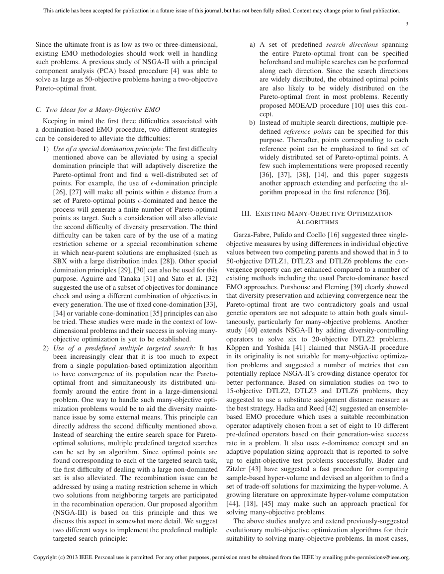
associate each population member with a reference point. For
this purpose, we define a reference line corresponding to each
reference point on the hyper-plane by joining the reference
point with the origin. Then, we calculate the perpendicular
distance of each population member of St from each of the
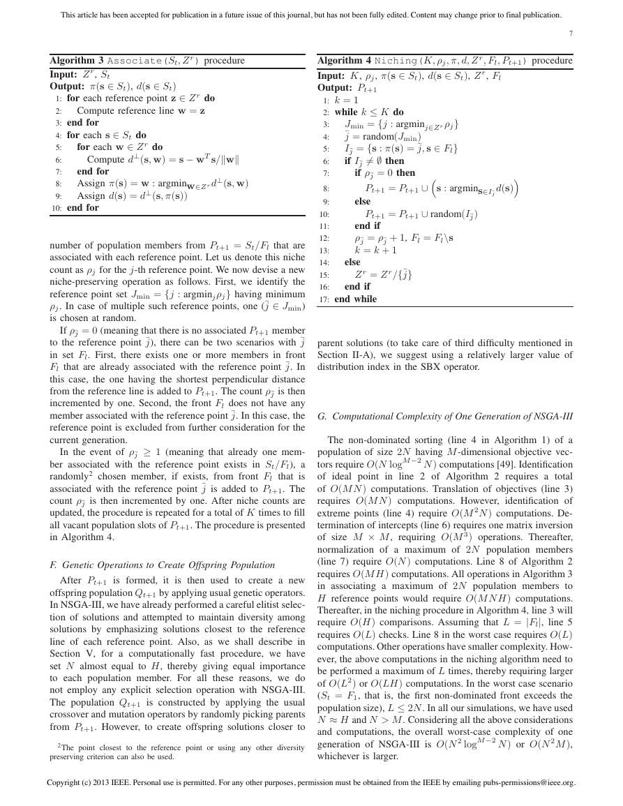
reference lines. The reference point whose reference line is
closest to a population member in the normalized objective
space is considered associated with the population member.
This is illustrated in Figure 3. The procedure is presented in
1.5
f3
1
0.5
0
0
0.5
f2
1
1.5
1.5
1
f1
0.5
0
Fig. 3. Association of population members with reference points is illustrated.
Algorithm 3.
E. Niche-Preservation Operation
It is worth noting that a reference point may have one
or more population members associated with it or need not
have any population member associated with it. We count the
Copyright (c) 2013 IEEE. Personal use is permitted. For any other purposes, permission must be obtained from the IEEE by emailing pubs-permissions@ieee.org.
�
This article has been accepted for publication in a future issue of this journal, but has not been fully edited. Content may change prior to final publication.
4:
5:
6:
7:
8:
9:
10:
11:
12:
13:
14:
15:
Algorithm 3 Associate(St, Z r) procedure
Input: Z r, St
Output: π(s ∈ St), d(s ∈ St)
1: for each reference point z ∈ Z r do
2:
3: end for
4: for each s ∈ St do
5:
Compute reference line w = z
for each w ∈ Z r do
Compute d⊥(s, w) = s − wT s/’w’
end for
Assign π(s) = w : argminw∈Zr d⊥(s, w)
Assign d(s) = d⊥(s,π (s))
6:
7:
8:
9:
10: end for
number of population members from Pt+1 = St/Fl that are
associated with each reference point. Let us denote this niche
count as ρj for the j-th reference point. We now devise a new
niche-preserving operation as follows. First, we identify the
reference point set Jmin = {j : argminjρj} having minimum
ρj. In case of multiple such reference points, one (¯j ∈ Jmin)
is chosen at random.
If ρ¯j = 0 (meaning that there is no associated Pt+1 member
to the reference point ¯j), there can be two scenarios with ¯j
in set Fl. First, there exists one or more members in front
Fl that are already associated with the reference point ¯j. In
this case, the one having the shortest perpendicular distance
from the reference line is added to Pt+1. The count ρ¯j is then
incremented by one. Second, the front Fl does not have any
member associated with the reference point ¯j. In this case, the
reference point is excluded from further consideration for the
current generation.
In the event of ρ¯j ≥ 1 (meaning that already one mem-
ber associated with the reference point exists in St/Fl), a
randomly2 chosen member, if exists, from front Fl
that is
associated with the reference point ¯j is added to Pt+1. The
count ρ¯j is then incremented by one. After niche counts are
updated, the procedure is repeated for a total of K times to fill
all vacant population slots of Pt+1. The procedure is presented
in Algorithm 4.
F. Genetic Operations to Create Offspring Population
After Pt+1 is formed, it
is then used to create a new
offspring population Qt+1 by applying usual genetic operators.
In NSGA-III, we have already performed a careful elitist selec-
tion of solutions and attempted to maintain diversity among
solutions by emphasizing solutions closest to the reference
line of each reference point. Also, as we shall describe in
Section V, for a computationally fast procedure, we have
set N almost equal to H, thereby giving equal importance
to each population member. For all these reasons, we do
not employ any explicit selection operation with NSGA-III.
The population Qt+1 is constructed by applying the usual
crossover and mutation operators by randomly picking parents
from Pt+1. However, to create offspring solutions closer to
2The point closest
to the reference point or using any other diversity
preserving criterion can also be used.
Algorithm 4 Niching(K, ρj,π, d, Z r, Fl, Pt+1) procedure
Input: K, ρj, π(s ∈ St), d(s ∈ St), Z r, Fl
Output: Pt+1
7
1: k = 1
2: while k ≤ K do
3:
Jmin = {j : argminj∈Zr ρj}
¯j = random(Jmin)
I¯j = {s : π(s) = ¯j, s ∈ Fl}
if I¯j )= ∅ then
if ρ¯j = 0 then
Pt+1 = Pt+1 ∪&s : argmins∈I¯j
d(s)’
else
Pt+1 = Pt+1 ∪ random(I¯j)
end if
ρ¯j = ρ¯j + 1, Fl = Fl\s
k = k + 1
else
Z r = Z r/{¯j}
end if
16:
17: end while
parent solutions (to take care of third difficulty mentioned in
Section II-A), we suggest using a relatively larger value of
distribution index in the SBX operator.
G. Computational Complexity of One Generation of NSGA-III
The non-dominated sorting (line 4 in Algorithm 1) of a
population of size 2N having M -dimensional objective vec-
tors require O(N logM−2 N ) computations [49]. Identification
of ideal point
in line 2 of Algorithm 2 requires a total
of O(M N ) computations. Translation of objectives (line 3)
requires O(M N ) computations. However, identification of
extreme points (line 4) require O(M 2N ) computations. De-
termination of intercepts (line 6) requires one matrix inversion
of size M × M , requiring O(M 3) operations. Thereafter,
normalization of a maximum of 2N population members
(line 7) require O(N ) computations. Line 8 of Algorithm 2
requires O(M H) computations. All operations in Algorithm 3
in associating a maximum of 2N population members to
H reference points would require O(M N H) computations.
Thereafter, in the niching procedure in Algorithm 4, line 3 will
require O(H) comparisons. Assuming that L = |Fl|, line 5
requires O(L) checks. Line 8 in the worst case requires O(L)
computations. Other operations have smaller complexity. How-
ever, the above computations in the niching algorithm need to
be performed a maximum of L times, thereby requiring larger
of O(L2) or O(LH) computations. In the worst case scenario
(St = F1, that is, the first non-dominated front exceeds the
population size), L ≤ 2N . In all our simulations, we have used
N ≈ H and N > M . Considering all the above considerations
and computations, the overall worst-case complexity of one
generation of NSGA-III is O(N 2 logM−2 N ) or O(N 2M ),
whichever is larger.
Copyright (c) 2013 IEEE. Personal use is permitted. For any other purposes, permission must be obtained from the IEEE by emailing pubs-permissions@ieee.org.
�
This article has been accepted for publication in a future issue of this journal, but has not been fully edited. Content may change prior to final publication.
8
III is set as the smallest multiple of four3 higher than H. For
MOEA/D procedures, we use a population size, N $ = H, as
suggested by their developers. For three-objective problems,
NUMBER OF REFERENCE POINTS/DIRECTIONS AND CORRESPONDING
POPULATION SIZES USED IN NSGA-III AND MOEA/D ALGORITHMS.
TABLE I
No. of
objectives
(M )
3
5
8
10
15
Ref. pts./
Ref. dirn.
(H)
91
210
156
275
135
popsize
NSGA-III MOEA/D
popsize
(N !)
91
210
156
275
135
(N )
92
212
156
276
136
12
$ or
we have used p = 12 in order to obtain H = #3−1+12
91 reference points (refer to equation 3). For five-objective
problems, we have used p = 6, so that H = 210 reference
points are obtained. Note that as long as p ≥ M is not chosen,
no intermediate point will be created by Das and Dennis’s
systematic approach. For eight-objective problems, even if we
use p = 8 (to have at least one intermediate reference point),
it requires 5,040 reference points. To avoid such a situation,
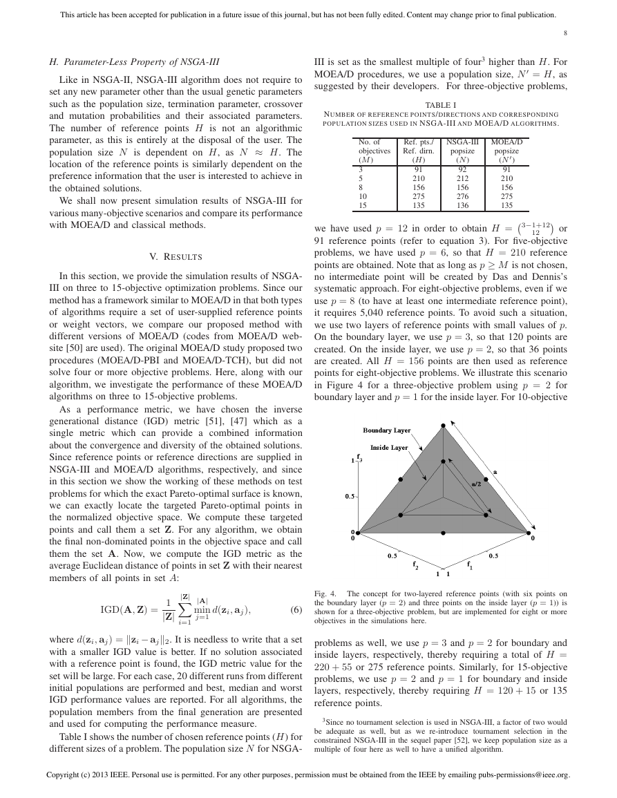
we use two layers of reference points with small values of p.
On the boundary layer, we use p = 3, so that 120 points are
created. On the inside layer, we use p = 2, so that 36 points
are created. All H = 156 points are then used as reference
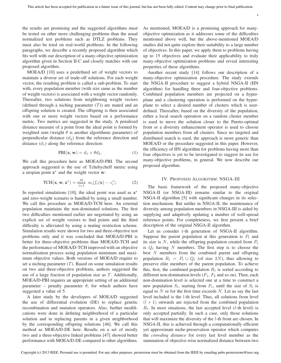
points for eight-objective problems. We illustrate this scenario
in Figure 4 for a three-objective problem using p = 2 for
boundary layer and p = 1 for the inside layer. For 10-objective
H. Parameter-Less Property of NSGA-III
Like in NSGA-II, NSGA-III algorithm does not require to
set any new parameter other than the usual genetic parameters
such as the population size, termination parameter, crossover
and mutation probabilities and their associated parameters.
The number of reference points H is not an algorithmic
parameter, as this is entirely at the disposal of the user. The
population size N is dependent on H, as N ≈ H. The
location of the reference points is similarly dependent on the
preference information that the user is interested to achieve in
the obtained solutions.
We shall now present simulation results of NSGA-III for
various many-objective scenarios and compare its performance
with MOEA/D and classical methods.
V. RESULTS
In this section, we provide the simulation results of NSGA-
III on three to 15-objective optimization problems. Since our
method has a framework similar to MOEA/D in that both types
of algorithms require a set of user-supplied reference points
or weight vectors, we compare our proposed method with
different versions of MOEA/D (codes from MOEA/D web-
site [50] are used). The original MOEA/D study proposed two
procedures (MOEA/D-PBI and MOEA/D-TCH), but did not
solve four or more objective problems. Here, along with our
algorithm, we investigate the performance of these MOEA/D
algorithms on three to 15-objective problems.
As a performance metric, we have chosen the inverse
generational distance (IGD) metric [51], [47] which as a
single metric which can provide a combined information
about the convergence and diversity of the obtained solutions.
Since reference points or reference directions are supplied in
NSGA-III and MOEA/D algorithms, respectively, and since
in this section we show the working of these methods on test
problems for which the exact Pareto-optimal surface is known,
we can exactly locate the targeted Pareto-optimal points in
the normalized objective space. We compute these targeted
points and call them a set Z. For any algorithm, we obtain
the final non-dominated points in the objective space and call
them the set A. Now, we compute the IGD metric as the
average Euclidean distance of points in set Z with their nearest
members of all points in set A:
IGD(A, Z) =
1
|Z|
|Z|
(i=1
|A|
min
j=1
d(zi, aj),
(6)
Fig. 4.
The concept for two-layered reference points (with six points on
the boundary layer (p = 2) and three points on the inside layer (p = 1)) is
shown for a three-objective problem, but are implemented for eight or more
objectives in the simulations here.
where d(zi, aj) = ’zi − aj’2. It is needless to write that a set
with a smaller IGD value is better. If no solution associated
with a reference point is found, the IGD metric value for the
set will be large. For each case, 20 different runs from different
initial populations are performed and best, median and worst
IGD performance values are reported. For all algorithms, the
population members from the final generation are presented
and used for computing the performance measure.
Table I shows the number of chosen reference points (H) for
different sizes of a problem. The population size N for NSGA-
problems as well, we use p = 3 and p = 2 for boundary and
inside layers, respectively, thereby requiring a total of H =
220 + 55 or 275 reference points. Similarly, for 15-objective
problems, we use p = 2 and p = 1 for boundary and inside
layers, respectively, thereby requiring H = 120 + 15 or 135
reference points.
3Since no tournament selection is used in NSGA-III, a factor of two would
be adequate as well, but as we re-introduce tournament selection in the
constrained NSGA-III in the sequel paper [52], we keep population size as a
multiple of four here as well to have a unified algorithm.
Copyright (c) 2013 IEEE. Personal use is permitted. For any other purposes, permission must be obtained from the IEEE by emailing pubs-permissions@ieee.org.
�


 2023年江西萍乡中考道德与法治真题及答案.doc
 2012年重庆南川中考生物真题及答案.doc
 2013年江西师范大学地理学综合及文艺理论基础考研真题.doc
 2020年四川甘孜小升初语文真题及答案I卷.doc
 2020年注册岩土工程师专业基础考试真题及答案.doc
 2023-2024学年福建省厦门市九年级上学期数学月考试题及答案.doc
 2021-2022学年辽宁省沈阳市大东区九年级上学期语文期末试题及答案.doc
 2022-2023学年北京东城区初三第一学期物理期末试卷及答案.doc
 2018上半年江西教师资格初中地理学科知识与教学能力真题及答案.doc
 2012年河北国家公务员申论考试真题及答案-省级.doc
 2020-2021学年江苏省扬州市江都区邵樊片九年级上学期数学第一次质量检测试题及答案.doc
 2022下半年黑龙江教师资格证中学综合素质真题及答案.doc