2010 International Conference on Pattern Recognition 2010 International Conference on Pattern Recognition 2010 International Conference on Pattern Recognition 2010 International Conference on Pattern Recognition 2010 International Conference on Pattern Recognition Image Segmentation Based on Adaptive Fuzzy-C-Means Clustering Mohamed Walid Ayech Karim El Kalti Bechir El Ayeb Pôle de Recherche en Faculté des Sciences de Pôle de Recherche en Informatique du Centre-Tunisie Monastir -Tunisie Informatique du Centre-Tunisie Email: ayechwalid@yahoo.fr Email: karim.kalti@gmail.com Email: ayeb_b@yahoo.com Abstract The clustering method “Fuzzy-C-Means” (FCM) is widely used in image segmentation. However, the major drawback of this method is its sensitivity to the noise. In this paper, we propose a variant of this method which aims at resolving this problem. Our approach is based on an adaptive distance which is calculated according to the spatial position of the pixel in the image. The obtained results have shown a significant improvement of our approach performance compared to the standard version of the FCM, especially regarding the robustness face to noise and the accuracy of the edges between regions. 1. Introduction Image segmentation constitutes an important step and an essential process of image analysis. Fuzzy-C- Means (FCM) [2] is one of the most popular unsupervised fuzzy clustering techniques that are applied with success in image segmentation. Although the original FCM algorithm yields good results for segmenting noise free images, it fails to segment images corrupted by noise or containing inaccurate edges. This sensitivity is essentially due to the absence of utilization of the information on the spatial position of pixels to be classified. Several authors tried to overcome this drawback by the integration of spatial information. Chuang [4] proposed a novel fuzzy clustering algorithm that uses a spatial membership degree representing the summation of the membership degree in the neighbourhood of each pixel. Tolias[5] developed a Sugeno type rule based system that imposes the membership degree of clustering results obtained after FCM algorithm. constraint by modifying spatial In our paper we propose a novel version of FCM that integrates the spatial information. The novelty the way of calculating concerns essentially the distance of similarity between the pixels of the image and the centers of the classes. The rest of this paper is organized as follows. Sections 2 and 3 present respectively the principle and the limits of the conventional FCM algorithm. In the following section we present our fuzzy clustering approach algorithm that image segmentation. Our segmentation method is tested on synthetic and MRI images. The results are illustrated and discussed in section 5. Finally, in section 6 we conclude the paper. 2. Fuzzy C Means Clustering incorporates a spatial constraint for Fuzzy-C-Means (FCM) clustering was developed by Bezdek [2]. It can be described as follows: Let X= {x1, x2, …, xn} denoted a set of n objects to be partitioned into C clusters, where each xj has d features. The FCM algorithm minimizes the objective function defined as follows: vxDu ( , ij i J ¦¦ (1) ) ( ) m C n j 1 i 1 j where: x uij represents the membership degree of jth object in the ith cluster, x vi represents the ith cluster center, x D represents a distance metric (generally the square of Euclidian distance) that measures the similarity between an object and a cluster center, x m •1 the degree of fuzzyfication. The membership degree of xj to the ith cluster is determined by calculating the gradient of J with respect to uij. Thus, these membership degrees are given by Equation 2: u ij § ¦C ¨ © 1 k  vxDvxD , ( ) ( , k j i  1  · 1  ¸ m 1 ¹ ) i (2) 1051-4651/10 $26.00 © 2010 IEEE 1051-4651/10 $26.00 © 2010 IEEE 1051-4651/10 $26.00 © 2010 IEEE 1051-4651/10 $26.00 © 2010 IEEE 1051-4651/10 $26.00 © 2010 IEEE DOI 10.1109/ICPR.2010.564 DOI 10.1109/ICPR.2010.564 DOI 10.1109/ICPR.2010.564 DOI 10.1109/ICPR.2010.564 DOI 10.1109/ICPR.2010.564 2298 2310 2306 2306 2306 

The cluster centers vi, i:1..C are determined by calculating the gradient of J with respect to vi. These centers are given by Equation 3: ) ¦ ¦ m ) u ( u ( x m n n (3) ij j v i j 1 ij j 1 The FCM algorithm can be summarized in the following steps: Step 1: Fix the cluster number and initialize the centers by random points from data set. Step 2: Update the membership degrees by using Equation 2 Step 3: Update centers using Equation 3. Step 4: Repeat steps 2 and 3 until convergence. The convergence of this algorithm will be reached when the change in membership values is less than a given threshold. 3. 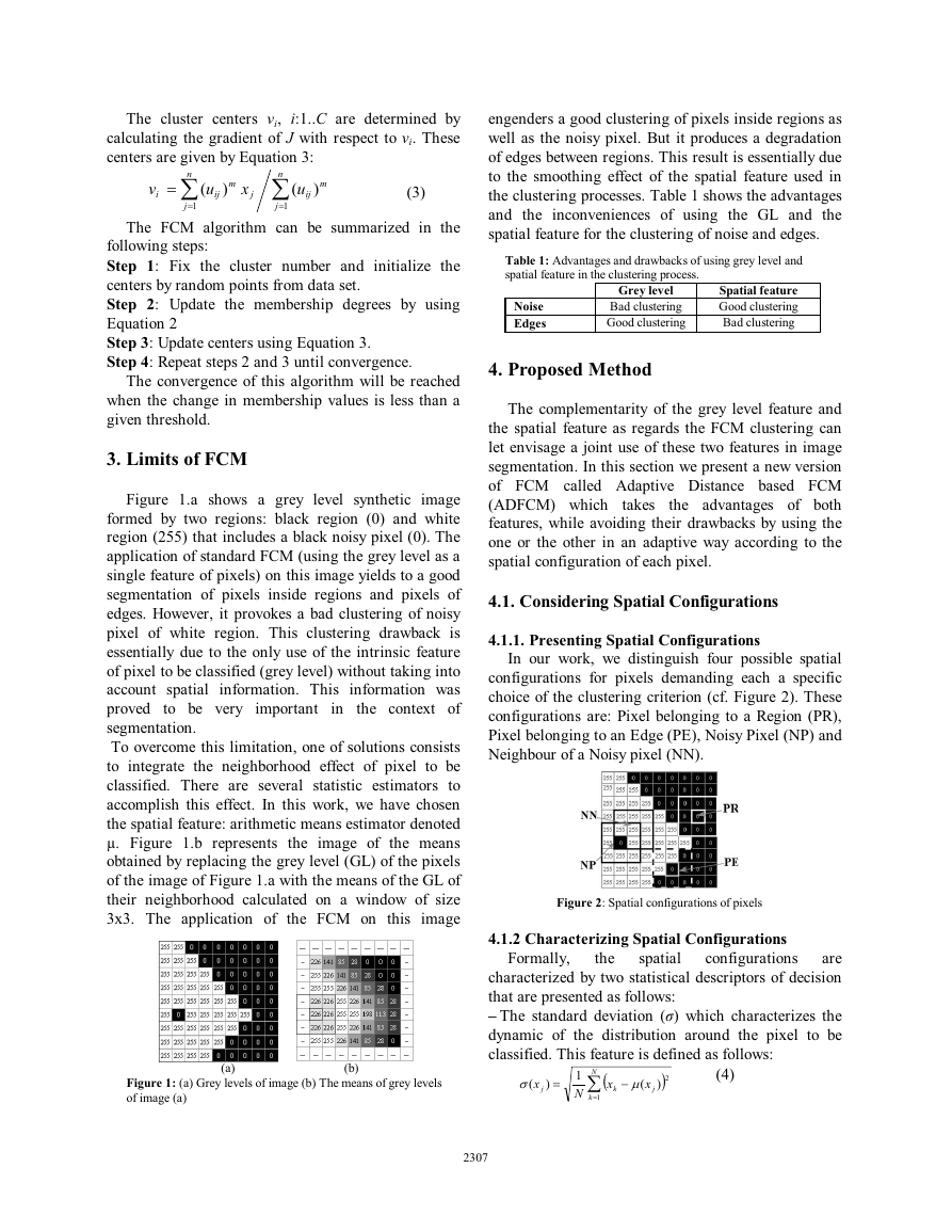Limits of FCM Figure 1.a shows a grey level synthetic image formed by two regions: black region (0) and white region (255) that includes a black noisy pixel (0). The application of standard FCM (using the grey level as a single feature of pixels) on this image yields to a good segmentation of pixels inside regions and pixels of edges. However, it provokes a bad clustering of noisy pixel of white region. This clustering drawback is essentially due to the only use of the intrinsic feature of pixel to be classified (grey level) without taking into account spatial information. This information was proved to be very important in the context of segmentation. To overcome this limitation, one of solutions consists to integrate the neighborhood effect of pixel to be classified. There are several statistic estimators to accomplish this effect. In this work, we have chosen the spatial feature: arithmetic means estimator denoted μ. Figure 1.b represents the image of the means obtained by replacing the grey level (GL) of the pixels of the image of Figure 1.a with the means of the GL of their neighborhood calculated on a window of size 3x3. The application of the FCM on this image (a) (b) Figure 1: (a) Grey levels of image (b) The means of grey levels of image (a) 2299 2311 2307 2307 2307 engenders a good clustering of pixels inside regions as well as the noisy pixel. But it produces a degradation of edges between regions. This result is essentially due to the smoothing effect of the spatial feature used in the clustering processes. Table 1 shows the advantages and the inconveniences of using the GL and the spatial feature for the clustering of noise and edges. Table 1: Advantages and drawbacks of using grey level and spatial feature in the clustering process. Noise Edges Grey level Bad clustering Good clustering Spatial feature Good clustering Bad clustering 4. Proposed Method The complementarity of the grey level feature and the spatial feature as regards the FCM clustering can let envisage a joint use of these two features in image segmentation. In this section we present a new version of FCM called Adaptive Distance based FCM (ADFCM) which the advantages of both features, while avoiding their drawbacks by using the one or the other in an adaptive way according to the spatial configuration of each pixel. takes 4.1. Considering Spatial Configurations 4.1.1. Presenting Spatial Configurations In our work, we distinguish four possible spatial configurations for pixels demanding each a specific choice of the clustering criterion (cf. Figure 2). These configurations are: Pixel belonging to a Region (PR), Pixel belonging to an Edge (PE), Noisy Pixel (NP) and Neighbour of a Noisy pixel (NN). Figure 2: Spatial configurations of pixels 4.1.2 Characterizing Spatial Configurations the spatial Formally, configurations are characterized by two statistical descriptors of decision that are presented as follows: – The standard deviation (ı) which characterizes the dynamic of the distribution around the pixel to be classified. This feature is defined as follows: (4) N V ( x ) j  x k 1 N ¦ k 1  P ( x j  2) 

– The knn which represents the number of the closest neighbours in term of grey levels with regard to the considered pixel. The knn is defined as follows: knn(xj) = Card{xpNeighborhood(xj) / |xp-xj|

Table 3: Misclassified pixels number inside and on the edges of regions of MRI cerebral image for the three tested techniques. FCM (GL) FCM (μ) ADFCM (Tı =55) 0 11 0 3 2 4 20 are experimented in the same conditions (a factor of fuzzyfication m = 2 and a convergence error = 0.001). The ADFCM uses as spatial feature the means μ calculated on an analysis window of size 3x3. in Figure 4.c. Conversely, Figure 4.a shows Panda image containing three classes of regions perfectly identified. Figure 4.b shows the result of applying the standard FCM to the original image using as a clustering criterion the grey levels. This result clearly illustrates the limitations of this method for the classification of noisy pixels. However, the application of the FCM based on the means feature can resolve the problem of noise as shown it engenders inaccurate edges segmentation (tree branches). The application of ADFCM (with Tı = 55) yields the segmentation shown in Figure 4.d. The three classes are correctly detected. This result confirms the good performance of the ADFCM compared to the standard FCM. Indeed, by using the adaptive distance, the ADFCM has achieved a compromise that allowed the reduction of noise while producing accurate edges. The visual result is supported by the statistics shown in Table 3 which gives the number of misclassified pixels inside and at edges of regions for each of the three classes that make up the image "Panda". Cerebral image segmentation consists in bounding three cerebral structures: grey matter (GM), white matter (WM) and the cerebrospinal fluid (CSF). Our tests are realized on the cerebral image of Figure 5.a. The application of the FCM based on the GL feature on this image gives noisy and overlapped classes particularly between both classes GM and WM (cf. Figure 4.b). The use of the FCM based on the spatial feature provokes a degradation of the obtained edges (cf. Figure 4.c). Whereas the use of the ADFCM for a threshold equal to 15 help enormously to reduce the noisy pixels while obtaining good identified regions (a) (d) Figure 4: Segmentation results using FCM (GL), FCM (μ) and ADFCM (Tı = 55) algorithms for Panda synthetic image. (b) (c) (a) (d) Figure 5: Segmentation results using FCM (GL), FCM (μ) and ADFCM (Tı = 15) algorithms for MRI cerebral image. (b) (c) 2301 2313 2309 2309 2309 Region Edge Region Edge Region Edge Classe1 Classe2 Classe3 Total 20 2 2 66 689 169 948 0 464 0 8 10 664 1146 and having continuous edges that are closer to the reality (cf. Figure 5.d). 6. Conclusion In this paper we have proposed a novel version of FCM based on dynamic and weighted similarity distance. Our approach is tested on synthetic and MRI cerebral images. The obtained results have shown a significant improvement of our approach performance compared to the standard FCM. The robustness face to noise and the accuracy of the edges between regions have been shown. However, the threshold Tı is strongly dependent on used images. This problem hasn’t been addressed in this paper and remains as further steps of research. References [1] A.K. Jain, M.N. Murty, P.J.Flynn, Data clustering: A review, ACM Computing surveys, Vol. 31, No. 3, pp. 264-323, 1999. the choice of [2] J.C. Bezdek, Pattern recognition with Fuzzy Objective Functions Algorithms, Plenum Press, New York, 1981. [3] L. Zadeh. Fuzzy sets, Information and control, Vol. 8, pp. 338-353, 1965. [4] K.S. Chuang, H.L. Tzeng, S. Chen, J. Wu. Fuzzy C Means Clustering with spatial information for image segmentation, Elsevier Science, Vol. 30, pp. 9-15, 2006. [5] Y.A. Tolias, S.M. Panas, On applying spatial constraints in fuzzy image clustering using a fuzzy rule based system, IEEE Signal Processing Letters, Vol. 5, pp. 245- 247, 1998. [6] D.L. Pham. Spatial models for fuzzy clustering, Computer vision and image understanding, Vol. 84, pp. 285-297, 2001. [7] D.J. Hemanth, D. Selvathi, J. Anitha. Effective fuzzy clustering algorithm for abnormal MR brain image segmentation, IEEE IACC, pp. 609-614, 2009.