论文研究 - 产生高时空分辨率归一化差异植被指数时间序列数据集的时空融合模型的比较.pdf

发布时间：2022-05-29 发布人：admin 分类：说明书资料大小：0.64M 资料格式：pdf 举报版权申诉

weixin_38553478-12436930-4744300845134210065.pdf-第1页.png

第1页 / 共7页

weixin_38553478-12436930-4744300845134210065.pdf-第2页.png

第2页 / 共7页

weixin_38553478-12436930-4744300845134210065.pdf-第3页.png

第3页 / 共7页

weixin_38553478-12436930-4744300845134210065.pdf-第4页.png

第4页 / 共7页

weixin_38553478-12436930-4744300845134210065.pdf-第5页.png

第5页 / 共7页

weixin_38553478-12436930-4744300845134210065.pdf-第6页.png

第6页 / 共7页

weixin_38553478-12436930-4744300845134210065.pdf-第7页.png

第7页 / 共7页

Comparison of Spatiotemporal Fusion Models for Producing High Spatiotemporal Resolution Normalized Difference Vegetation Index Time Series Data Sets

Abstract

Keywords

1. Introduction

2. Materials and Methods

2.1. Study site and Data Preparation

2.2. Selected Spatiotemporal Fusion Models

2.2.1. STARFM

2.2.2. ESTARFM

2.2.3. FSDAF

2.2.4. STVIFM

2.3. Assessing Prediction Accuracy

3. Result and Discussion

3.1. Prediction Performance

3.2. Quantitative Assessment

4. Conclusion

Conflicts of Interest

References

Journal of Computer and Communications, 2019, 7, 65-71 http://www.scirp.org/journal/jcc ISSN Online: 2327-5227 ISSN Print: 2327-5219 Comparison of Spatiotemporal Fusion Models for Producing High Spatiotemporal Resolution Normalized Difference Vegetation Index Time Series Data Sets Zhizhong Han1, Wenya Zhao2 1College of Computer Science and Technology, Chongqing University of Posts and Telecommunications, Chongqing, China 2Chongqing Aerospace Poly Technic, Chongqing, China How to cite this paper: Han, Z.Z. and Zhao, W.Y. (2019) Comparison of Spati- otemporal Fusion Models for Producing High Spatiotemporal Resolution Norma- lized Difference Vegetation Index Time Series Data Sets. Journal of Computer and Communications, 7, 65-71. https://doi.org/10.4236/jcc.2019.77007 Received: May 15, 2019 Accepted: July 7, 2019 Published: July 10, 2019 Abstract It has a great significance to combine multi-source with different spatial res- olution and temporal resolution to produce high spatiotemporal resolution Normalized Difference Vegetation Index (NDVI) time series data sets. In this study, four spatiotemporal fusion models were analyzed and compared with each other. The models included the spatial and temporal adaptive reflectance model (STARFM), the enhanced spatial and temporal adaptive reflectance fu- sion model (ESTARFM), the flexible spatiotemporal data fusion model (FSDAF), and a spatiotemporal vegetation index image fusion model (STVIFM). The objective of is to: 1) compare four fusion models using Land- sat-MODIS NDVI image from the Banan district, Chongqing Province; 2) analyze the prediction accuracy quantitatively and visually. Results indicate that STVIFM would be more suitable to produce NDVI time series data sets. Keywords Spatiotemporal Fusion, NDVI, Time Series, STVIFM 1. Introduction The Normalized Difference Vegetation Index (NDVI) is a widely used vegeta- tion index (VI) and provides a way of evaluating the biophysical or biochemical information related to vegetation growth [1]. Long term NDVI time-series data- sets have been widely used for monitoring ecosystem dynamics to understand the responses of climate change [2] [3]. However, due to financial and technical DOI: 10.4236/jcc.2019.77007 Jul. 10, 2019 65 Journal of Computer and Communications

Z. Z. Han, W. Y. Zhao constraints, it is difficult to obtain NDVI data with both high spatial and high temporal resolution on the same remote sensing instrument [4]. In addition, long periods of cloud cover problems in some regions have aggravated this mat- ter [5]. Thus, spatiotemporal fusion techniques which combine NDVI date from multi-sensors with high spatial and temporal resolution is feasible solution to acquire remote sensing time series for monitoring surface vegetations dynamics [6] [7]. Up to now, several spatiotemporal fusion models have been proposed. Gao et al. [8] proposed a spatial and temporal adaptive reflectance fusion model (STARFM) to blend MODIS and Landsat image to produce a synthetic surface reflectance product at 30 m spatial resolution. Based the STARFM, Zhu et al. [9] developed an enhanced spatial and temporal adaptive reflectance fusion model (ESTARFM), introducing conversion coefficient between pixels and improving the prediction accuracy. Zhu et al. [10] proposed the flexible spatiotemporal data fusion model (FSDAF) which performs better in predicting abrupt land cover changes. Liao et al. [11] developed a spatiotemporal vegetation index image fu- sion model (STVIFM) to generate NDVI time series images with high spatial and temporal resolution in heterogeneous regions. In this study, we made a comparation between STARFM, ESTARFM, FSDAF, and STVIFM methods, tested by Landsat and MODIS data acquired in same site and quantitatively as- sess the accuracy of predicted image generated from each fusion model. 2. Materials and Methods 2.1. 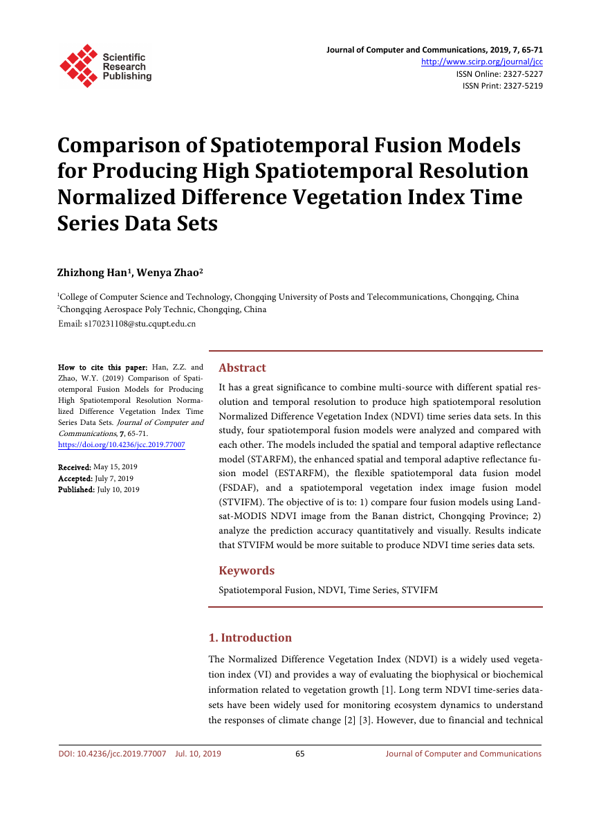Study site and Data Preparation In this study, a selected study area is shown in Figure 1, which located in Banan District (29˚34'10''N, 106˚57'35''E) in Chongqing Province to perform the com- parison between the spatiotemporal fusion models. We select MODIS daily sur- face reflectance image and Landsat-8 image acquired for these dates during this period: April 28, 2015, August 02, 2015, and October 21, 2015. 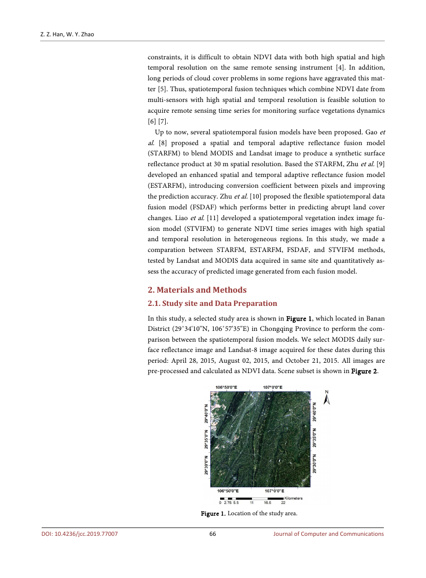All images are pre-processed and calculated as NDVI data. Scene subset is shown in Figure 2. DOI: 10.4236/jcc.2019.77007 Figure 1. Location of the study area. 66 Journal of Computer and Communications

Z. Z. Han, W. Y. Zhao Figure 2. Landsat NDVI (upper row) and MODIS NDVI (lower row) images. From left to right, they were acquired from April 28, 2015, August 02, 2015, and October 21, 2015, respectively. 2.2. Selected Spatiotemporal Fusion Models 2.2.1. STARFM The STARFM is based on the moving window technology, which requires at least a pair of high-resolution image and coarse-resolution image on the base time and one coarse-resolution image on the predicted time. By introducing a weigh function using spectral difference, temporal difference and spatial differ- ence to determining the contribution of other pixels in the window to the central pixel. And then a synthetic high Spatiotemporal image (F(t2)) is predicted with the high- and coarse-resolution data through the proposed weight function. This model can be written as in Equation (1). F t ( 2) = ∑ Wi F t M t ( 1) ( 2) + ( − M t ( 1)) (1) where, F(t1) and M(t1) denote the high-and coarse resolution date on the base date, M(t2) is the coarse resolution date at the predicted date, and Wi is the weight function. 2.2.2. ESTARFM The ESTARFM needs at least two pairs of high-resolution image and coarse res- olution image on the base time and one coarse-resolution image on the pre- dicted time. Compared with STARFM, this method not only considers the spa- tial and spectral similarity between pixels, but also introduces a conversion coef- ficient, which is derived from the high-and coarse-resolution data during the observation period using a linear regression. The final high-resolution predic- tion is computed as in Equation (2). F t ( 2) = ∑ Wi Vi F t M t * ( ( 1) ( 2) + − M t ( 1)) (2) DOI: 10.4236/jcc.2019.77007 67 Journal of Computer and Communications

Z. Z. Han, W. Y. Zhao where, F(t1) and M(t1) denote the high-and coarse resolution data on the base date, M(t2) is the coarse resolution data at the predicted date, and Wi, Vi denote the weight function and conversion coefficient respectively. 2.2.3. FSDAF The FSDAF using one pair of high-resolution image and coarse-resolution im- age on the base time and one coarse-resolution image on the predicted time, and it also need to use land cover map. This model integrates STARFM, the linear unmixing method [12] and the thin plate spline (TPS) interpolator that main- tains the land cover change signals and local variability, which combined the temporal prediction from the linear unmixing method with the spatial predic- tion obtained by the TPS and distribute the residual to fine pixel to get the final prediction. It can be written as Equation (3). F t ( 2) = F t ( 1) + ∆∑ F * Wi (3) where, F(t1), F(t2) denote the high-resolution image on the base time and pre- dicted time respectively. F∆ is referred to the change between t1 and t2, which computed by the linear unmixing method and TPS. And Wi is the weight func- tion. 2.2.4. STVIFM The STVIFM requires two pairs of high- and coarse-resolution images acquired on the base time and one coarse-resolution on the predicted date. On the one hand, this model links the mean NDVI change of high-resolution pixels to mean NDVI change of coarse resolution pixels within a moving window. On the other hand, it also considers the difference in NDVI change rates at different growing stages. And the final prediction can be written as Equation (4). * NDVI NDVI( 2) NDVI( 1) (4) ∆∑ Wi = t t + where, NDVI(t2), NDVI(t1) are the high-resolution date on the prediction time and base time respectively. ΔNDVI denote the change between t1 and t2, which calculated by this model. And the Wi is the weight function. 2.3. Assessing Prediction Accuracy The model’s prediction performance is quantitatively evaluated by representative metrics. And the r and RMSE (root mean squared errors) are used to measure the difference between the predicted image and actual image. The formulations of these metrics are as follows: r = ∑ ∑ ( N j 1 = N j 1 = ( x j − x j − 2 x ) x y )( ∑ N j = − y ) j ( y j 2 − y ) (5) 2 DOI: 10.4236/jcc.2019.77007 RMSE = − y j 2 ) ∑ N j = 1( x j N (6) 68 Journal of Computer and Communications

Z. Z. Han, W. Y. Zhao where N is the total number of pixels in the predicted image, xj and yj are the values of the jth pixel in the predicted image and the actual image respectively. And x , y represent the mean gray values of the predicted image and the ac- tual image respectively. 3. Result and Discussion 3.1. 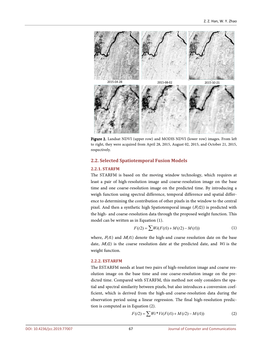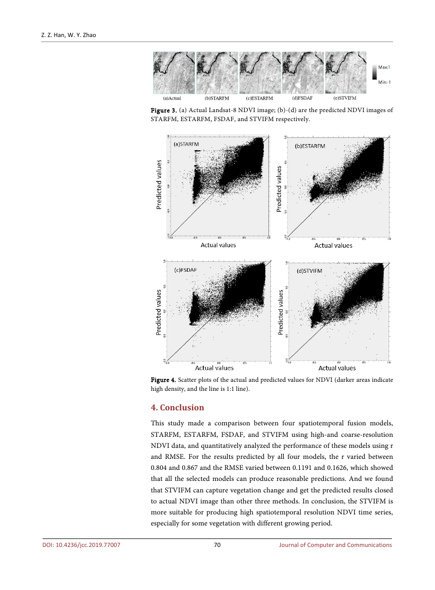Prediction Performance We use the August 02 Landsat NDVI image as validation source and use April 28 and October 21 to predict the August 02 image. Figure 3 shows the actual NDVI image and predicted NDVI image by four spatiotemporal fusion models on August 02, 2015. All the predicted NDVI images are consistent with the ac- tual image from visual comparison, and water boundaries and clear land can be predicted obviously, which demonstrate the practicality of these spatiotemporal models. 3.2. 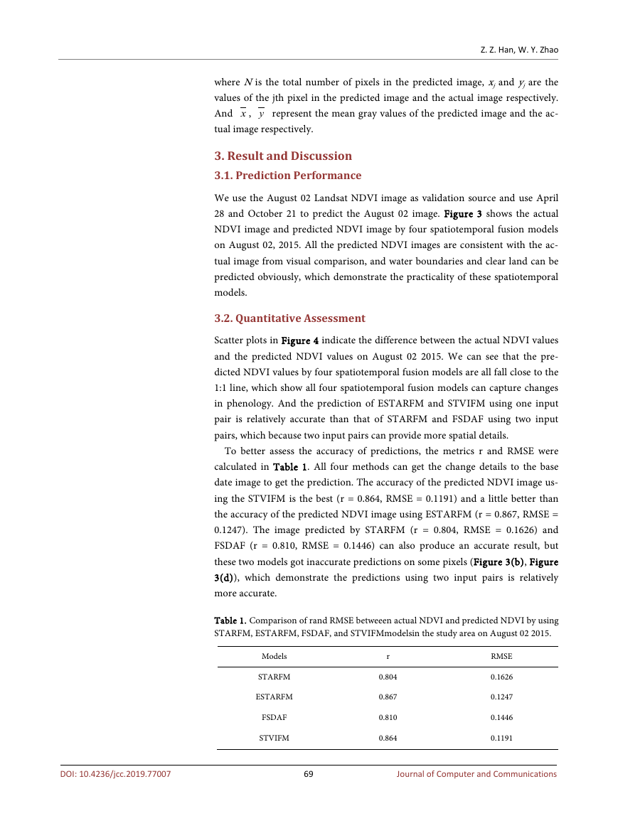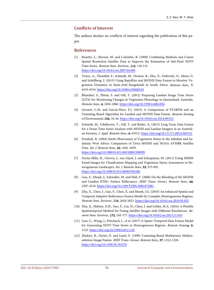Quantitative Assessment Scatter plots in Figure 4 indicate the difference between the actual NDVI values and the predicted NDVI values on August 02 2015. We can see that the pre- dicted NDVI values by four spatiotemporal fusion models are all fall close to the 1:1 line, which show all four spatiotemporal fusion models can capture changes in phenology. And the prediction of ESTARFM and STVIFM using one input pair is relatively accurate than that of STARFM and FSDAF using two input pairs, which because two input pairs can provide more spatial details. To better assess the accuracy of predictions, the metrics r and RMSE were calculated in Table 1. All four methods can get the change details to the base date image to get the prediction. The accuracy of the predicted NDVI image us- ing the STVIFM is the best (r = 0.864, RMSE = 0.1191) and a little better than the accuracy of the predicted NDVI image using ESTARFM (r = 0.867, RMSE = 0.1247). The image predicted by STARFM (r = 0.804, RMSE = 0.1626) and FSDAF (r = 0.810, RMSE = 0.1446) can also produce an accurate result, but these two models got inaccurate predictions on some pixels (Figure 3(b), Figure 3(d)), which demonstrate the predictions using two input pairs is relatively more accurate. Table 1. Comparison of rand RMSE betweeen actual NDVI and predicted NDVI by using STARFM, ESTARFM, FSDAF, and STVIFMmodelsin the study area on August 02 2015. Models STARFM ESTARFM FSDAF STVIFM r 0.804 0.867 0.810 0.864 RMSE 0.1626 0.1247 0.1446 0.1191 69 Journal of Computer and Communications DOI: 10.4236/jcc.2019.77007

Z. Z. Han, W. Y. Zhao Figure 3. (a) Actual Landsat-8 NDVI image; (b)-(d) are the predicted NDVI images of STARFM, ESTARFM, FSDAF, and STVIFM respectively. Figure 4. Scatter plots of the actual and predicted values for NDVI (darker areas indicate high density, and the line is 1:1 line). 4. Conclusion This study made a comparison between four spatiotemporal fusion models, STARFM, ESTARFM, FSDAF, and STVIFM using high-and coarse-resolution NDVI data, and quantitatively analyzed the performance of these models using r and RMSE. For the results predicted by all four models, the r varied between 0.804 and 0.867 and the RMSE varied between 0.1191 and 0.1626, which showed that all the selected models can produce reasonable predictions. And we found that STVIFM can capture vegetation change and get the predicted results closed to actual NDVI image than other three methods. In conclusion, the STVIFM is more suitable for producing high spatiotemporal resolution NDVI time series, especially for some vegetation with different growing period. 70 Journal of Computer and Communications DOI: 10.4236/jcc.2019.77007

Z. Z. Han, W. Y. Zhao Conflicts of Interest The authors declare no conflicts of interest regarding the publication of this pa- per. References [1] Busetto, L., Meroni, M. and Colombo, R. (2008) Combining Medium and Coarse Spatial Resolution Satellite Data to Improve the Estimation of Sub-Pixel NDVI Time Series. Remote Sens. Environ., 112, 118-131. https://doi.org/10.1016/j.rse.2007.04.004 [2] Tewes, A., Thonfeld, F., Schmidt, M., Oomen, R., Zhu, X., Dubovyk, O., Menz, G. and Schellberg, J. (2015) Using RapidEye and MODIS Data Fusion to Monitor Ve- getation Dynamics in Semi-Arid Rangelands in South Africa. Remote Sens., 7, 6510-6534. https://doi.org/10.3390/rs70606510 [3] Bhandari, S., Phinn, S. and Gill, T. (2012) Preparing Landsat Image Time Series (LITS) for Monitoring Changes in Vegetation Phenology in Queensland, Australia. Remote Sens., 4, 1856-1886. https://doi.org/10.3390/rs4061856 [4] Gevaert, C.M. and García-Haro, F.J. (2015) A Comparison of STARFM and an Unmixing Based Algorithm for Landsat and MODIS Data Fusion. Remote Sensing of Environment, 156, 34-44. https://doi.org/10.1016/j.rse.2014.09.012 [5] Schmidt, M., Udelhoven, T., Gill, T. and Röder, A. (2012) Long Term Data Fusion for a Dense Time Series Analysis with MODIS and Landsat Imagery in an Australi- an Savanna. J. Appl. Remote Sens., 6, 63512. https://doi.org/10.1117/1.JRS.6.063512 [6] Fensholt, R. (2004) Earth Observation of Vegetation Status in the Sahelian and Su- danian West Africa: Comparison of Terra MODIS and NOAA AVHRR Satellite Data. Int. J. Remote Sens., 25, 1641-1659. https://doi.org/10.1080/01431160310001598999 [7] Zurita-Milla, R., Clevers, J., van Gijsel, J. and Schaepman, M. (2011) Using MERIS Fused Images for Classification Mapping and Vegetation Status Assessment in He- terogeneous Landscapes. Int. J. Remote Sens., 32, 973-991. https://doi.org/10.1080/01431160903505286 [8] Gao, F., Masek, J., Schwaller, M. and Hall, F. (2006) On the Blending of the MODIS and Landsat ETM+ Surface Reflectance. IEEE Trans. Geosci. Remote Sens., 44, 2207-2218. https://doi.org/10.1109/TGRS.2006.872081 [9] Zhu, X., Chen, J., Gao, F., Chen, X. and Masek, J.G. (2010) An enhanced Spatial and Temporal Adaptive Reflectance Fusion Model for Complex Heterogeneous Regions. Remote Sens. Environ., 114, 2610-2623. https://doi.org/10.1016/j.rse.2010.05.032 [10] Zhu, X., Helmer, E.H., Gao, F., Liu, D., Chen, J. and Lefsky, M.A. (2016) A Flexible Spatiotemporal Method for Fusing Satellite Images with Different Resolutions. Re- mote Sens. Environ., 172, 165-177. https://doi.org/10.1016/j.rse.2015.11.016 [11] Liao, C., Wang, J., Pritchard, I., et al. (2017) A Spatio-Temporal Data Fusion Model for Generating NDVI Time Series in Heterogeneous Regions. Remote Sensing, 9, 1125. https://doi.org/10.3390/rs9111125 [12] Zhukov, B., Oertel, D. and Lanzl, F. (1999) Unmixing-Based Multisensor Multire- solution Image Fusion. IEEE Trans. Geosci. Remote Sens., 37, 1212-1226. https://doi.org/10.1109/36.763276 71 Journal of Computer and Communications DOI: 10.4236/jcc.2019.77007

分享到：

赞收藏

资料库

论文研究 - 产生高时空分辨率归一化差异植被指数时间序列数据集的时空融合模型的比较.pdf

相关推荐

开发技术

热门标签

最新资料