MAXIMUM LIKELIHOOD ESTIMATION OF THE
COX-INGERSOLL-ROSS PROCESS: THE MATLAB
IMPLEMENTATION
Kamil Klad´ıvko1
Department of Statistics and Probability Calculus, University of Economics, Prague
and Debt Management Department, Ministry of Finance of the Czech Republic
kladivk@vse.cz or kamil.kladivko@mfcr.cz
Abstract
The square root diffusion process is widely used for modeling interest rates
behaviour.
It is an underlying process of the well-known Cox-Ingersoll-Ross
term structure model (1985). We investigate maximum likelihood estimation
of the square root process (CIR process) for interest rate time series. The
MATLAB implementation of the estimation routine is provided and tested on
the PRIBOR 3M time series.
1 CIR Process for Interest Rate Modeling
A continuous-time model in finance typically rest on one or more stationary diffusion processes
{Xt, t ≥ 0}, with dynamics represented by stochastic differential equations:
(1)
where {Wt, t ≥ 0} is a standard Brownian motion. The functions µ(·) and σ2(·) are, respectively,
the drift and the diffusion functions of the process.
dXt = µ(Xt)dt + σ(Xt)dWt,
The fundamental process in interest rate modeling is the square root process given by the
following stochastic differential equation:
√
drt = α(µ − rt)dt +
(2)
where rt is the interest rate and θ ≡ (α, µ, σ) are model parameters. The drift function µ(rt, θ) =
α(µ − rt) is linear and possess a mean reverting property, i.e.
interest rate rt moves in the
direction of its mean µ at speed α. The diffusion function σ2(rt, θ) = rtσ2 is proportional to the
interest rate rt and ensures that the process stays on a positive domain.
rtσdWt,
The square root process (2) is the basis for the Cox, Ingersoll, and Ross short-term interest
rate model [1] and therefore often denoted as the CIR process in the financial literature.
1.1 CIR process densities
If α, µ, σ are all positive and 2αµ ≥ σ2 holds, the CIR process is well-defined and has a steady
state (marginal) distribution. The marginal density is gamma distributed.
For maximum likelihood estimation of the parameter vector θ ≡ (α, µ, σ) transition den-
sities are required. The CIR process is one of few cases, among the diffusion processes, where
the transition density has a closed form expression. We follow the notation given in [1] on page
391. Given rt at time t the density of rt+∆t at time t + ∆t is
p(rt+∆t|rt; θ, ∆t) = ce−u−v( v
u
1This work was supported by grant of IGA VSE nr. IG410046
√
) q
2 Iq(2
uv),
(3)
�
where
σ2(1 − e−α∆t) ,
2α
c =
u = crte−α∆t,
v = crt+∆t,
2αµ
σ2 − 1,
q =
√
and Iq(2
(3) has been originally derived in [2].
uv) is modified Bessel function of the first kind and of order q. The transition density
Sometimes, it is particularly useful to work with a transformation st+∆t = 2crt+∆t. We
can easily derive that the transition density of st+∆t is
g(st+∆t|st; θ, ∆t) = g(2crt+∆t|2crt; θ, ∆t) =
p(rt+∆t|rt; θ, ∆t),
1
2c
(4)
which is the the noncentral χ2 distribution with 2q + 2 degrees of freedom and non-centrality
parameter 2u.
2 Maximum Likelihood Implementation in MATLAB
Parameter estimation is carried out on interest rate time series with N observations {rti, i =
1 . . . N}. We consider equally spaced observations with ∆t time step.
2.1 Likelihood function
The likelihood function for interest rate time series with N observations is
It is computationally convenient to work with the log-likelihood function
L(θ) =
p(rti+1|rti; θ, ∆t).
N−1Y
i=1
N−1X
(5)
(6)
(7)
utivti+1)}
,
from which we easily derive the log-likelihood function of the CIR process
ln L(θ) =
i=1
ln p(rti+1|rti; θ, ∆t),
vti+1
−uti − vti+1 + 0.5q ln
N−1X
i=1
+ ln{Iq(2√
uti
ln L(θ) = (N − 1) ln c +
where uti = crtie−α∆t and vti+1 = crti+1. We find maximum likelihood estimates ˆθ of parameter
vector θ by maximizing the log-likelihood function (7) over its parameter space:
ˆθ ≡ (ˆα, ˆµ, ˆσ) = arg max
θ
ln L(θ).
(8)
Since the logarithmic function is monotonically increasing, maximizing the log-likelihood func-
tion also maximizes the likelihood function.
For solving optimization problem (8) we have to rely on numerical solution. The function
fminsearch, which is a standard part of MATLAB, makes the job. The function fminsearch
is an implementation of Nelder-Mead simplex method, see MATLAB help for details.
�
2.2 Initial estimates
For convergence to the global optimum initial (starting) points of optimization are crucial. We
suggest to use Ordinary Least Squares (OLS) on discretized version of (2):
rt+∆t − rt = α(µ − rt)∆t + σ
rtεt,
(9)
√
where εt is normally distributed with zero mean and variance ∆t, more precisely εt is a white
noise process. For performing OLS we transform (9) into:
The drift initial estimates are found by minimizing the OLS objective function
which is solved by
√
− α
rt∆t + σεt.
rt+∆t − rt
√
rt
= αµ∆t√
rt
N−1X
N 2 − 2N + 1 +
α,µ
i=1
rti
rti+1 − rti
√
N−1P
(bα,bµ) = arg min
− αµ∆t√
rti
N−1P
N−1P
− N−1P
N−1P
N 2 − 2N + 1 − N−1P
rti+1 − N−1P
(N − 1)
− N−1P
N−1P
N−1P
N−1P
rti+1
rti
rti+1
1
rti
rti
rti
i=1
i=1
i=1
i=1
i=1
i=1
rti
rti+1
1
rti
N 2 − 2N + 1 +
bα =
bµ =
(10)
(11)
(12)
(13)
,
.
!2
√
+ α
rti∆t
,
i=1
i=1
1
rti
1
rti
∆t
!
− (N − 1)
N−1P
N−1P
rti
− (N − 1)
i=1
1
rti
N−1P
i=1
rti+1
rti
N−1P
rti+1
rti
The diffusion parameter initial estimate bσ is found as a standard deviation of residuals.
i=1
i=1
i=1
i=1
i=1
The practical MATLAB implementation can, of course, rely on a back slash operator (\)
which automatically performs OLS and yields the same results as (12) and (13):
% CIR initial parameters estimation
x = Model.Data(1:end-1); % Time series of interest rates observations
dx = diff(Model.Data);
dx = dx./x.^0.5;
regressors = [Model.TimeStep./x.^0.5, Model.TimeStep*x.^0.5];
drift = regressors\dx; % OLS regressors coefficients estimates
res = regressors*drift - dx;
alpha = -drift(2);
mu = -drift(1)/drift(2);
sigma = sqrt(var(res, 1)/Model.TimeStep);
InitialParams = [alpha mu sigma]; % Vector of initial parameters
The initial estimates (bα,bµ,bσ) are starting points for maximizing the log-likelihood func-
tion (7)
2.3 Implementing the log-likelihood function using the command besseli
For implementing the objective function (7) we need to evaluate the modified Bessel function
√
of the first kind Iq(2
uv) is available under the command
besseli(q, 2*sqrt(u.*v)) in MATLAB but direct usage of this function results in an esti-
√
mation failure. The reason is that the Bessel function Iq(2
uv) approaches rapidly to the
√
uv). The Bessel function Iq(2
�
plus infinity and optimization routines (e.g. fminsearch, fmincon) are not able to handle this
problem.2
Fortunately there is a scaled version of the Bessel function in MATLAB which we denote
√
q (2
uv) and is available under the command besseli(q, 2*sqrt(u.*v), 1). The I 1
uv)
√
I 1
uv) and therefore solves the problem of the rapid divergence. We
equals Iq(2
accordingly adjust the objective function (7) into
√
q (2
√
uv) exp(−2
N−1X
i=1
ln L = (N − 1) ln c +
−uti − vti+1 + 0.5q ln
vti+1
uti
+ ln{I 1
q (2√
utivti+1)} + 2√
utivti+1
.
(14)
The MATLAB code of the log-likelihood function can look as follows:
CIR process using the MATLAB besseli function
function lnL = CIRobjective1(Params, Model)
% =========================================================================
% PURPOSE : Log-likelihood objective function (multiplied by -1) for the
%
% =========================================================================
% USAGE
%
%
% =========================================================================
% RETURNS : lnL
% =========================================================================
= Delta t
= Time series of interest rates observations
= Model parameters (alpha, mu, sigma)
= Objective function value
Model.Data
Params
: Model.TimeStep
Data = Model.Data;
DataF = Data(2:end);
DataL = Data(1:end-1);
Nobs = length(Data);
TimeStep = Model.TimeStep;
alpha = Params(1);
mu = Params(2);
sigma = Params(3);
c = 2*alpha/(sigma^2*(1-exp(-alpha*TimeStep)));
q = 2*alpha*mu/sigma^2-1;
u = c*exp(-alpha*TimeStep)*DataL;
v = c*DataF;
z = 2*sqrt(u.*v);
bf = besseli(q,z,1);
lnL= -(Nobs-1)*log(c) + sum(u + v - 0.5*q*log(v./u) - log(bf) - z);
end
2.4 Implementing the log-likelihood function using the command ncx2pdf
There is an alternative way to implement the log-likelihood function in MATLAB and that is
by using directly the noncentral χ2 probability density function (pdf) which is available in the
Statistics Toolbox under the command ncx2pdf. The function ncx2pdf relyes on an alternative
definition of the noncentral χ2 pdf. The alternative definition of the noncentral χ2 pdf does not
use the modified Bessel function of the first kind but is based on the central χ2 distribution
√
2We already can encounter this problem when calculating the transition density (3). On one hand the Bessel
uv) approaches rapidly to the plus infinity, on the other hand the term exp(−u − v) approaches
function Iq(2
rapidly to the minus infinity and that causes calculation crash.
�
weighted by Poisson distribution3.
In this alternative implementation we use the random variable transformation given by
(4). We call ncx2pdf(s, 2*q+2, 2.*u), where s = 2crt+∆t are the transformed interest rate
values. The MATLAB code of the log-likelihood function can look as follows:
CIR process using MATLAB ncx2pdf function.
function lnL = CIRobjective2(Params, Model)
% =========================================================================
% PURPOSE : Log-likelihood objective function (multiplied by -1) for the
%
% =========================================================================
% USAGE
%
%
% =========================================================================
% RETURNS : lnL
% =========================================================================
= Delta t
= Time series of interest rates observations
= Model parameters (alpha, mu, sigma)
: Model.TimeStep
Model.Data
Params
= Objective function value
Data = Model.Data;
DataF = Data(2:end);
DataL = Data(1:end-1);
TimeStep = Model.TimeStep;
alpha = Params(1);
mu = Params(2);
sigma = Params(3);
c = 2*alpha/(sigma^2*(1-exp(-alpha*TimeStep)));
q = 2*alpha*mu/sigma^2-1;
u = c*exp(-alpha*TimeStep)*DataL;
v = c*DataF;
s = 2*c*DataF;
nc = 2*u; % noncentrality parameter
df = 2*q+2; % degrees of freedom
gpdf = ncx2pdf(s, df, nc);
ppdf = 2*c*gpdf;
lnL = sum(-log(ppdf));
end
2.5 Optimization
The minimization of the negative of the log-likelihood function can be achieved by the fminsearch
function. Both suggested implementation of the log-likelihood function work equally well with
only slight differences in results. The ncx2pdf implementation is generally more time consuming.
Both implementations of the log-likelihood are available under CIRobjective1.m, respec-
tively, CIRobjective2.m. The optimization routine (initial estimates and optimization itself) is
implemented under CIRestimation.m.
3Details can be found at http://en.wikipedia.org/wiki/Noncentral chi distribution or by reading the
ncx2pdf source code.
�
3 Estimating the CIR Process for PRIBOR 3M
We present the results of estimating the CIR process for times series of daily (business days)
observations of PRIBOR 3M from 3 January 1994 to 4 October 2007. As our data are sampled
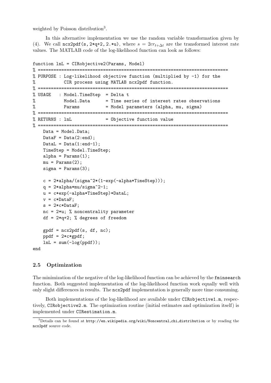
each business day, we set the time step ∆t = 1/250. Time series of PRIBOR 3M is plotted in
Figure 1.
Figure 1: Time series of PRIBOR 3M from 1/3/1994 through 10/4/2007. Interest rate
in percents.
3.1 Estimation results
The estimation results reports Table 1. In this particular case the OLS results are noticeably
different from the maximum likelihood (ML) results which is not a common outcome for other
interest rates data sets. It is caused by jumps of PRIBOR 3M in 1997. It is, of course, arguable
whether the CIR process is a right choice for the given PRIBOR 3M data set but this is not our
concern in this paper. Using either implementation of the log-likelihood function returns results
which differ on the fourth decimal number.
OLS (initial)
ML besseli
ML ncx2pdf
ˆα
0.1209
0.4363
0.4360
ˆµ
0.0423
0.0613
0.0612
ˆσ
0.1642
0.1491
0.1492
ln L
4.7140
4.7080
Table 1: This table reports the OLS and maximum likelihood (ML) results for daily
(business day) PRIBOR 3M data set from 3 January 1994 to 4 October 2007. Time
step ∆t = 1/250. The ln L refers to the maximized value of the log-likelihood divided
by the number of observations.
3.2 The optimization propagation and the log-likelihood
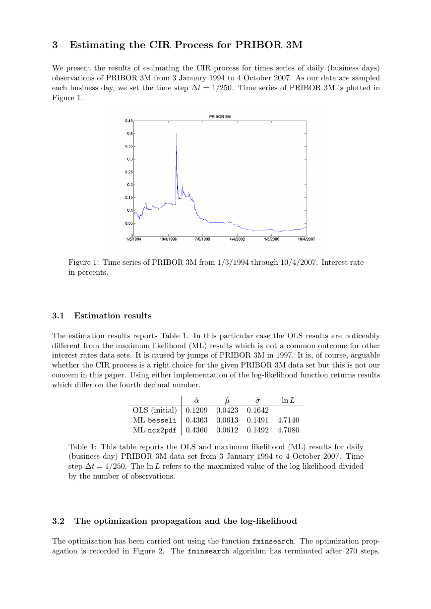
The optimization has been carried out using the function fminsearch. The optimization prop-
agation is recorded in Figure 2. The fminsearch algorithm has terminated after 270 steps.
�
Figure 2: Optimization propagation for the PRIBOR 3M data set. The upper graph
plots parameters propagation, the lower graph log-likelihood propagation.
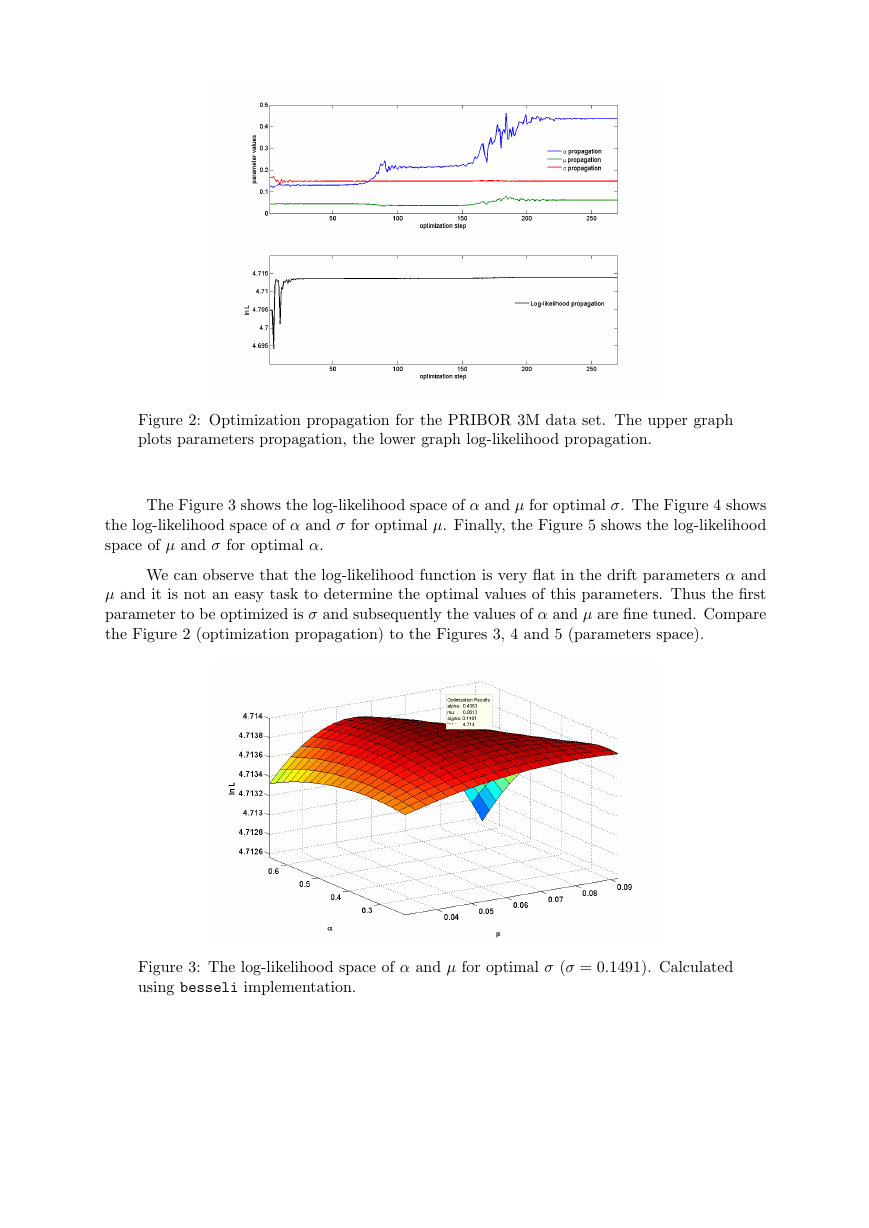
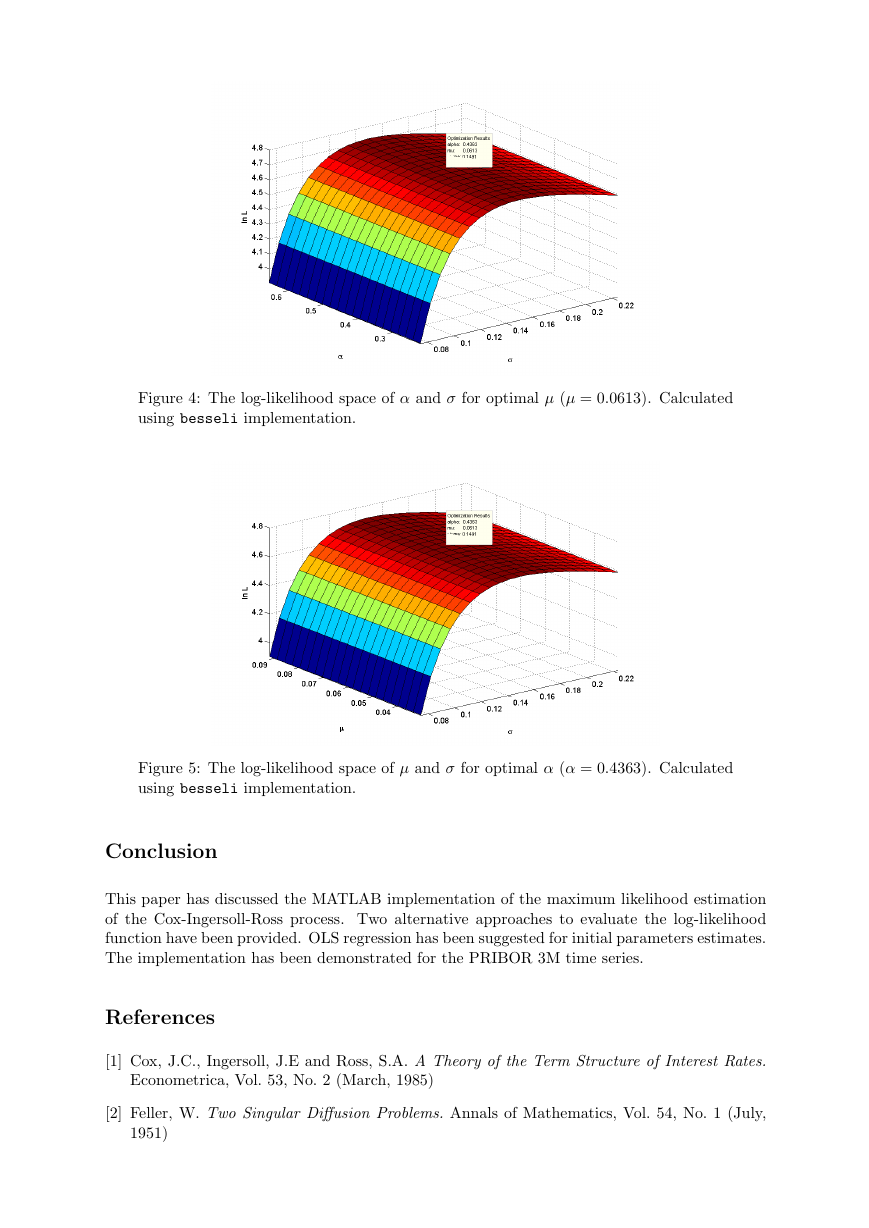
The Figure 3 shows the log-likelihood space of α and µ for optimal σ. The Figure 4 shows
the log-likelihood space of α and σ for optimal µ. Finally, the Figure 5 shows the log-likelihood
space of µ and σ for optimal α.
We can observe that the log-likelihood function is very flat in the drift parameters α and
µ and it is not an easy task to determine the optimal values of this parameters. Thus the first
parameter to be optimized is σ and subsequently the values of α and µ are fine tuned. Compare
the Figure 2 (optimization propagation) to the Figures 3, 4 and 5 (parameters space).
Figure 3: The log-likelihood space of α and µ for optimal σ (σ = 0.1491). Calculated
using besseli implementation.
�
Figure 4: The log-likelihood space of α and σ for optimal µ (µ = 0.0613). Calculated
using besseli implementation.
Figure 5: The log-likelihood space of µ and σ for optimal α (α = 0.4363). Calculated
using besseli implementation.
Conclusion
This paper has discussed the MATLAB implementation of the maximum likelihood estimation
of the Cox-Ingersoll-Ross process. Two alternative approaches to evaluate the log-likelihood
function have been provided. OLS regression has been suggested for initial parameters estimates.
The implementation has been demonstrated for the PRIBOR 3M time series.
References
[1] Cox, J.C., Ingersoll, J.E and Ross, S.A. A Theory of the Term Structure of Interest Rates.
Econometrica, Vol. 53, No. 2 (March, 1985)
[2] Feller, W. Two Singular Diffusion Problems. Annals of Mathematics, Vol. 54, No. 1 (July,
1951)
�


 2023年江西萍乡中考道德与法治真题及答案.doc
 2012年重庆南川中考生物真题及答案.doc
 2013年江西师范大学地理学综合及文艺理论基础考研真题.doc
 2020年四川甘孜小升初语文真题及答案I卷.doc
 2020年注册岩土工程师专业基础考试真题及答案.doc
 2023-2024学年福建省厦门市九年级上学期数学月考试题及答案.doc
 2021-2022学年辽宁省沈阳市大东区九年级上学期语文期末试题及答案.doc
 2022-2023学年北京东城区初三第一学期物理期末试卷及答案.doc
 2018上半年江西教师资格初中地理学科知识与教学能力真题及答案.doc
 2012年河北国家公务员申论考试真题及答案-省级.doc
 2020-2021学年江苏省扬州市江都区邵樊片九年级上学期数学第一次质量检测试题及答案.doc
 2022下半年黑龙江教师资格证中学综合素质真题及答案.doc