Feature Denoising for Improving Adversarial Robustness
Cihang Xie1,2∗
Yuxin Wu2
1Johns Hopkins University
Laurens van der Maaten2
Alan Yuille1
2Facebook AI Research
Kaiming He2
9
1
0
2
r
a
M
5
2
]
V
C
.
s
c
[
2
v
1
1
4
3
0
.
2
1
8
1
:
v
i
X
r
a
Abstract
Adversarial attacks to image classification systems
present challenges to convolutional networks and oppor-
tunities for understanding them. This study suggests that
adversarial perturbations on images lead to noise in the
features constructed by these networks. Motivated by this
observation, we develop new network architectures that
increase adversarial robustness by performing feature
denoising. Specifically, our networks contain blocks that
denoise the features using non-local means or other filters;
the entire networks are trained end-to-end. When combined
with adversarial training, our feature denoising networks
substantially improve the state-of-the-art in adversarial
robustness in both white-box and black-box attack set-
tings. On ImageNet, under 10-iteration PGD white-box
attacks where prior art has 27.9% accuracy, our method
achieves 55.7%; even under extreme 2000-iteration PGD
white-box attacks, our method secures 42.6% accuracy.
Our method was ranked first in Competition on Adversarial
Attacks and Defenses (CAAD) 2018 — it achieved 50.6%
classification accuracy on a secret,
ImageNet-like test
dataset against 48 unknown attackers, surpassing the
runner-up approach by ∼10%.
Code is available at
https://github.com/facebookresearch/
ImageNet-Adversarial-Training.
1. Introduction
Adversarial attacks to image classification systems [20]
add small perturbations to images that lead these systems
into making incorrect predictions. While the perturba-
tions are often imperceptible or perceived as small “noise”
in the image,
these attacks are highly effective against
even the most successful convolutional network based sys-
tems [11, 14]. The success of adversarial attacks leads to
security threats in real-world applications of convolutional
networks, but equally importantly, it demonstrates that these
networks perform computations that are dramatically differ-
ent from those in human brains.
Figure 1 shows a randomly selected feature map of a
ResNet [9] applied on a clean image (top) and on its ad-
∗Work done during an internship at Facebook AI Research.
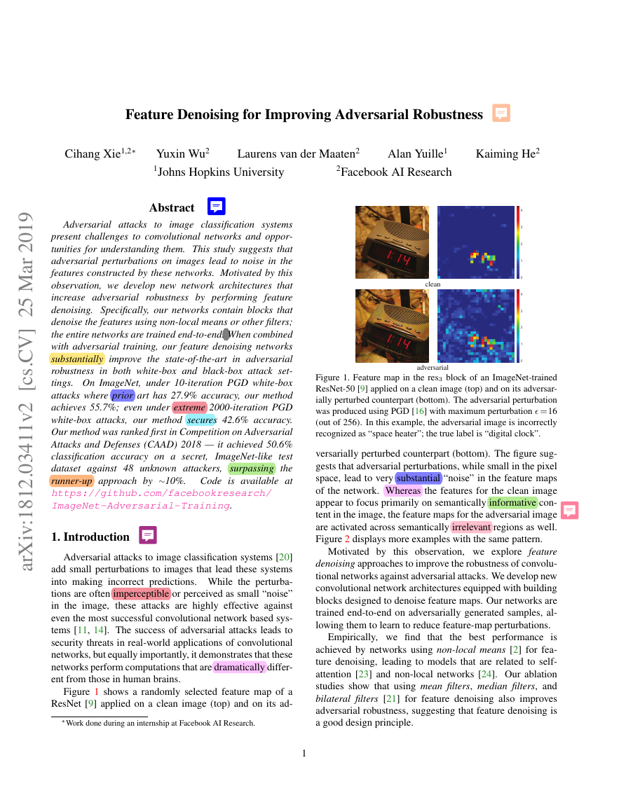
Figure 1. Feature map in the res3 block of an ImageNet-trained
ResNet-50 [9] applied on a clean image (top) and on its adversar-
ially perturbed counterpart (bottom). The adversarial perturbation
was produced using PGD [16] with maximum perturbation � =16
(out of 256). In this example, the adversarial image is incorrectly
recognized as “space heater”; the true label is “digital clock”.
versarially perturbed counterpart (bottom). The figure sug-
gests that adversarial perturbations, while small in the pixel
space, lead to very substantial “noise” in the feature maps
of the network. Whereas the features for the clean image
appear to focus primarily on semantically informative con-
tent in the image, the feature maps for the adversarial image
are activated across semantically irrelevant regions as well.
Figure 2 displays more examples with the same pattern.
Motivated by this observation, we explore feature
denoising approaches to improve the robustness of convolu-
tional networks against adversarial attacks. We develop new
convolutional network architectures equipped with building
blocks designed to denoise feature maps. Our networks are
trained end-to-end on adversarially generated samples, al-
lowing them to learn to reduce feature-map perturbations.
Empirically, we find that
the best performance is
achieved by networks using non-local means [2] for fea-
ture denoising, leading to models that are related to self-
attention [23] and non-local networks [24]. Our ablation
studies show that using mean filters, median filters, and
bilateral filters [21] for feature denoising also improves
adversarial robustness, suggesting that feature denoising is
a good design principle.
1
01234cleanadversarial01234�
Figure 2. More examples similar to Figure 1. We show feature maps corresponding to clean images (top) and to their adversarial perturbed
versions (bottom). The feature maps for each pair of examples are from the same channel of a res3 block in the same ResNet-50 trained on
clean images. The attacker has a maximum perturbation � = 16 in the pixel domain.
Our models outperform the state-of-the-art in adversarial
robustness against highly challenging white-box attacks on
ImageNet [18]. Under 10-iteration PGD attacks [16], we
report 55.7% classification accuracy on ImageNet, largely
surpassing the prior art’s 27.9% [10] with the same at-
tack protocol. Even when faced with extremely challeng-
ing 2000-iteration PGD attacks that have not been ex-
plored in other literature, our model achieves 42.6% accu-
racy. Our ablation experiments also demonstrate that fea-
ture denoising consistently improves adversarial defense re-
sults in white-box settings.
Our networks are also highly effective under the black-
box attack setting. The network based on our method won
the defense track in the recent Competition on Adversarial
Attacks and Defenses (CAAD) 2018, achieving 50.6% ac-
curacy against 48 unknown attackers, under a strict “all-or-
nothing” criterion. This is an 10% absolute (20% relative)
accuracy increase compared to the CAAD 2018 runner-up
model. We also conduct ablation experiments in which we
defend against the five strongest attackers from CAAD 2017
[13], demonstrating the potential of feature denoising.
2. Related Work
training
networks
by
Adversarial
training [6, 10, 16] defends against
perturbations
on
adversarial
images that are generated on-the-fly dur-
adversarial
ing training. Adversarial training constitutes the current
state-of-the-art in adversarial robustness against white-box
attacks; we use it to train our networks. Adversarial logit
paring (ALP) [10] is a type of adversarial training that
encourages the logit predictions of a network for a clean
image and its adversarial counterpart to be similar. ALP
can be interpreted as “denoising” the logit predictions for
the adversarial image, using the logits for the clean image
as the “noise-free” reference.
Other approaches to increase adversarial robustness in-
clude pixel denoising. Liao et al. [15] propose to use high-
level features to guide the pixel denoiser; in contrast, our
denoising is applied directly on features. Guo et al. [8]
transform the images via non-differentiable image prepro-
cessing, like image quilting [4], total variance minimiza-
tion [17], and quantization. While these defenses may be
effective in black-box settings, they can be circumvented
in white-box settings because the attacker can approximate
the gradients of their non-differentiable computations [1].
In contrast to [8], our feature denoising models are differ-
entiable, but are still able to improve adversarial robustness
against very strong white-box attacks.
3. Feature Noise
Adversarial images are created by adding perturbations
to images, constraining the magnitude of perturbations to
be small in terms of a certain norm (e.g., L∞ or L2). The
perturbations are assumed to be either imperceptible by hu-
mans, or perceived as noise that does not impede human
recognition of the visual content. Although the perturba-
tions are constrained to be small at the pixel level, no such
constraints are imposed at the feature level in convolutional
networks. Indeed, the perturbation of the features induced
by an adversarial image gradually increases as the image is
propagated through the network [15, 8], and non-existing
activations in the feature maps are hallucinated.
In other
words, the transformations performed by the layers in the
network exacerbate the perturbation, and the hallucinated
activations can overwhelm the activations due to the true
signal, which leads the network to make wrong predictions.
We qualitatively demonstrate these characteristics of
adversarial images by visualizing the feature maps they give
rise to. Given a clean image and its adversarially perturbed
counterpart, we use the same network (here, a ResNet-50
[9]) to compute its activations in the hidden layers. Figure 1
and 2 show typical examples of the same feature map on
clean and adversarial images, extracted from the middle of
the network (in particular, from a res3 block). These figures
01234012340123012301230123cleanadversarial�
Figure 4. A generic denoising block. It wraps the denoising oper-
ation (e.g., non-local means, bilateral, mean, median filters) with
a 1×1 convolution and an identity skip connection [9].
4. Denoising Feature Maps
Motivated by the empirical observations above, we pro-
pose to improve adversarial robustness by adding denoising
blocks at intermediate layers of convolutional networks.
The denoising blocks are trained jointly with all layers
of the network in an end-to-end manner using adversarial
training. The end-to-end adversarial training allows the re-
sulting networks to (partly) eliminate feature map noise that
is data-dependent, i.e., noise that is generated by the at-
tacker. It also naturally handles the noise across multiple
layers by considering how changes in earlier layers may im-
pact the feature/noise distributions of later layers.
Empirically, we find that the best-performed denoising
blocks are inspired by self-attention transformers [23] that
are commonly used in machine translation and by non-local
networks [24] that are used for video classification. In this
study, we focus on the design of denoising blocks and study
their denoising effects. Besides non-local means, we also
experiment with simpler denoising operations such as bilat-
eral filtering, mean filtering, and median filtering inside our
convolutional networks.
4.1. Denoising Block
Figure 4 shows the generic form of our denoising block.
The input to the block can be any feature layer in the convo-
lutional neural network. The denoising block processes the
input features by a denoising operation, such as non-local
means or other variants. The denoised representation is first
processed by a 1×1 convolutional layer, and then added to
the block’s input via a residual connection [9].1
The design in Figure 4 is inspired by self-attention [23]
and non-local blocks [24]. However, only the non-local
means [2] operation in the denoising block is actually doing
the denoising; the 1×1 convolutions and the residual con-
nection are mainly for feature combination. While various
operations can suppress noise, they can also impact signal.
The usage of the residual connection can help the network
1In our terminology, a “denoising operation” refers to the computa-
tion that only performs denoising (blue box in Figure 4), and a “denoising
block” refers to the entire block (all of Figure 4).
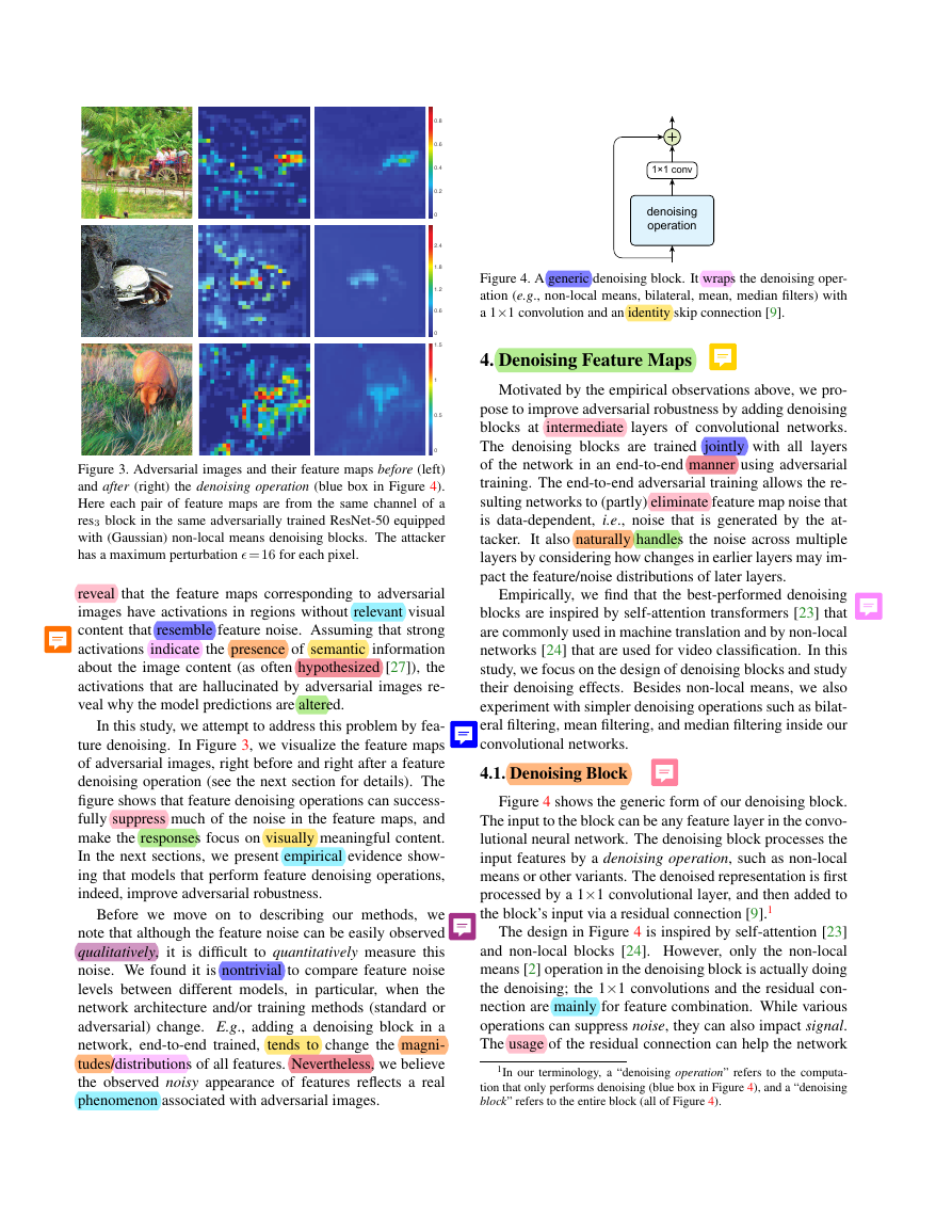
Figure 3. Adversarial images and their feature maps before (left)
and after (right) the denoising operation (blue box in Figure 4).
Here each pair of feature maps are from the same channel of a
res3 block in the same adversarially trained ResNet-50 equipped
with (Gaussian) non-local means denoising blocks. The attacker
has a maximum perturbation � = 16 for each pixel.
reveal that the feature maps corresponding to adversarial
images have activations in regions without relevant visual
content that resemble feature noise. Assuming that strong
activations indicate the presence of semantic information
about the image content (as often hypothesized [27]), the
activations that are hallucinated by adversarial images re-
veal why the model predictions are altered.
In this study, we attempt to address this problem by fea-
ture denoising. In Figure 3, we visualize the feature maps
of adversarial images, right before and right after a feature
denoising operation (see the next section for details). The
figure shows that feature denoising operations can success-
fully suppress much of the noise in the feature maps, and
make the responses focus on visually meaningful content.
In the next sections, we present empirical evidence show-
ing that models that perform feature denoising operations,
indeed, improve adversarial robustness.
Before we move on to describing our methods, we
note that although the feature noise can be easily observed
qualitatively, it is difficult to quantitatively measure this
noise. We found it is nontrivial to compare feature noise
levels between different models, in particular, when the
network architecture and/or training methods (standard or
adversarial) change. E.g., adding a denoising block in a
network, end-to-end trained, tends to change the magni-
tudes/distributions of all features. Nevertheless, we believe
the observed noisy appearance of features reflects a real
phenomenon associated with adversarial images.
00.20.40.60.800.511.500.61.21.82.41×1 convdenoisingoperation�
to retain signals, and the tradeoff between removing noise
and retaining signal is adjusted by the 1×1 convolution,
which is learned end-to-end with the entire network. We
will present ablation studies showing that both the residual
connection and the 1×1 convolution contribute to the effec-
tiveness of the denoising block. The generic form of the
denoising block allows us to explore various denoising op-
erations, as introduced next.
4.2. Denoising Operations
We experiment with four different instantiations of the
denoising operation in our denoising blocks.
Non-local means. Non-local means [2] compute a de-
noised feature map y of an input feature map x by taking
a weighted mean of features in all spatial locations L:
yi =
1
C(x)
f (xi, xj) · xj,
(1)
∀j∈L
where f (xi, xj) is a feature-dependent weighting function
and C(x) is a normalization function. We note that the
weighted average in Eqn. (1) is over xj, rather than another
embedding of xj, unlike [23, 24] — denoising is directly
on the input feature x, and the correspondence between the
feature channels in y and x is kept. Following [24], we con-
sider two forms:
• Gaussian (softmax) sets f (xi, xj) = e
1√
d
ber of channels, and C =∀j∈L f (xi, xj). By notic-
θ(xi)Tφ(xj ),
where θ(x) and φ(x) are two embedded versions of
x (obtained by two 1×1 convolutions), d is the num-
ing that f /C is the softmax function, this version is
shown in [24] to be equivalent to the softmax-based,
self-attention computation of [23].
• Dot product sets f (xi, xj) = xT
i xj and C(x) = N,
where N is the number of pixels in x. Unlike the
Gaussian non-local means, the weights of the weighted
mean do not sum up to 1 in dot-product non-local
means. However, qualitative evaluations suggest it
does suppress noise in the features. Experiments also
show this version improves adversarial robustness. In-
terestingly, we find that it is unnecessary to embed x
in the dot-product version of non-local means for the
model to work well. This is unlike the Gaussian non-
local means, in which embedding is essential. The dot-
product version provides a denoising operation with no
extra parameters (blue box in Figure 5).
Figure 5, adapted from [24], shows the implementation of
the denoising block based on non-local means.
Bilateral filter. It is easy to turn the non-local means in
Eqn. (1) into a “local mean”. Doing so leads to the classi-
cal bilateral filter [21] that is popular for edge-preserving
Figure 5. A block with non-local means as its denoising operation.
The blue part illustrates the implementation of non-local means in
Eqn. (1). The shapes of the feature tensors are noted, with cor-
responding reshaping/transposing performed: here, H and W are
the height and width of the feature maps, and we use 256 chan-
nels as an example. If softmax is used, it is the Gaussian version
(with appropriate 1×1 convolution embeddings used; omitted in
this figure); if softmax is not used, it is the dot product version.
denoising. Formally, it is defined as:
∀j∈Ω(i)
yi =
1
C(x)
f (xi, xj) · xj.
(2)
This equation only differs from Eqn. (1) in the neighbor-
hood, Ω(i), which is a local region (e.g., a 3×3 patch)
around pixel i. In Eqn. (2), we consider the Gaussian and
dot product implementations of the weights as before.
Mean filter. Perhaps the simplest form of denoising is the
mean filter (average pooling with a stride of 1). Mean filters
reduce noise but also smooth structures, so it is reasonable
to expect them to perform worse than the above weighted
means. However, somewhat surprisingly, experiments show
that denoising blocks using mean filters as the denoising
operation can still improve adversarial robustness.
Median filter. Lastly, we consider an interesting denoising
filter that has rarely been used in deep networks: median
filtering. The median filter is defined as:
yi = median{∀j ∈ Ω(i) : xj},
(3)
where the median is over a local region, Ω(i), and is per-
formed separately for each channel. Median filters are
known to be good at removing salt-and-pepper noise and
outliers of similar kind. Training convolutional networks
that contain median filters is an open problem, but we find
experimentally that using median filters as a denoising op-
eration can also improve adversarial robustness.
In summary, our study explores a rich collection of
denoising operations. Sec. 6 reports the results for all the
denoising operations described above.
1×1 convH×W×256HW×256256×HWHW×HWHW×256HW×256H×W×256H×W×256x(softmax)�
5. Adversarial Training
6. Experiments
We show the effectiveness of feature denoising on top of
very strong baselines. Our strong experimental results are
partly driven by a successful implementation of adversarial
training [6, 16]. In this section, we describe our implemen-
tation of adversarial training, which is used for training both
baseline models and our feature denoising models.
The basic idea of adversarial training [6, 16] is to train
the network on adversarially perturbed images. The ad-
versarially perturbed images can be generated by a given
white-box attacker based on the current parameters of the
models. We use the Projected Gradient Descent (PGD)2
[16] as the white-box attacker for adversarial training.
PGD attacker. PGD is an iterative attacker. At each itera-
tion, it performs a gradient descent step in the loss function
w.r.t. the image pixel values, based on an adversarially se-
lected output target. Next, it projects the resulting perturbed
images into the feasible solution space — within a maxi-
mum per-pixel perturbation of � of the clean image (that is,
subject to an L∞ constraint). The hyper-parameters of the
PGD attacker during adversarial training are: the maximum
perturbation for each pixel � = 16, the attack step size α = 1,
and the number of attack iterations n = 30. For this PGD
in adversarial training, we can initialize the adversarial im-
age by the clean image, or randomly within the allowed �
[16]. We randomly choose from both initializations in the
PGD attacker during adversarial training: 20% of training
batches use clean images to initialize PGD, and 80% use
random points within the allowed �.
Distributed training with adversarial images. For each
mini-batch, we use PGD to generate adversarial images for
that mini-batch. Then we perform a one-step SGD on these
perturbed images and update the model weights. Our SGD
update is based exclusively on adversarial images; the mini-
batch contains no clean images.
Because a single SGD update is preceded by n-step
PGD (with n = 30), the total amount of computation in
adversarial training is ∼n× bigger than standard (clean)
training. To make adversarial training practical, we per-
form distributed training using synchronized SGD on 128
GPUs. Each mini-batch contains 32 images per GPU (i.e.,
the total mini-batch size is 128×32 = 4096). We follow the
training recipe of [7]3 to train models with such large mini-
batches. On ImageNet, our models are trained for a total of
110 epochs; we decrease the learning rate by 10× at the 35-
th, 70-th, and 95-th epoch. A label smoothing [19] of 0.1 is
used. The total time needed for adversarial training on 128
Nvidia V100 GPUs is approximately 38 hours for the base-
line ResNet-101 model, and approximately 52 hours for the
baseline ResNet-152 model.
2Publicly available: https://github.com/MadryLab/cifar10_challenge
3Implemented using the publicly available Tensorpack framework [25].
We evaluate feature denoising on the ImageNet classi-
fication dataset [18] that has ∼1.28 million images in 1000
classes. Following common protocols [1, 10] for adversarial
images on ImageNet, we consider targeted attacks when
evaluating under the white-box settings, where the targeted
class is selected uniformly at random; targeted attacks are
also used in our adversarial training. We evaluate top-1
classification accuracy on the 50k ImageNet validation im-
ages that are adversarially perturbed by the attacker (regard-
less of its targets), also following [1, 10].
In this paper, adversarial perturbation is considered un-
der L∞ norm (i.e., maximum difference for each pixel),
with an allowed maximum value of �. The value of � is
relative to the pixel intensity scale of 256.
Our baselines are ResNet-101/152 [9]. By default, we
add 4 denoising blocks to a ResNet: each is added after the
last residual block of res2, res3, res4, and res5, respectively.
6.1. Against White-box Attacks
Following the protocol of ALP [10], we report defense
results against PGD as the white-box attacker.4 We evaluate
with � =16, a challenging case for defenders on ImageNet.
Following [16], the PGD white-box attacker initializes
the adversarial perturbation from a random point within the
allowed � cube. We set its step size α = 1, except for 10-
iteration attacks where α is set to �/10 = 1.6. We consider a
numbers of PGD attack iterations ranging from 10 to 2000.
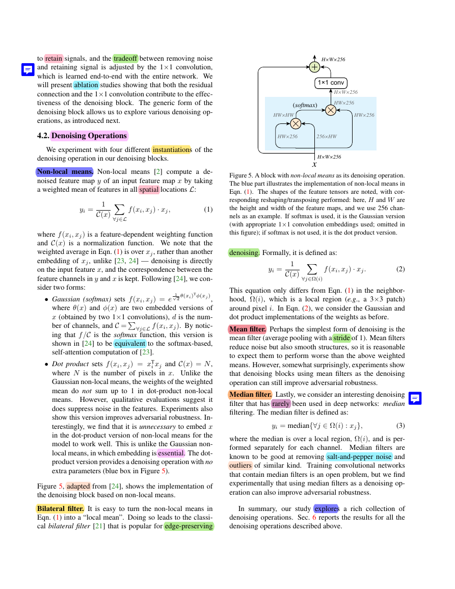
Main results. Figure 6 shows the main results. We first
compare with ALP [10], the previous state-of-the-art. ALP
was evaluated under 10-iteration PGD attack in [10], on
Inception-v3 [19]. It achieves 27.9% accuracy on ImageNet
validation images (Figure 6, purple triangle).
ResNet-101 and ResNet-152 in Figure 6 are our baseline
models (without any denoising blocks) trained using our
adversarial training implementation. Even with the lower-
capacity model of R-101, our baseline is very strong — it
has 49.7% accuracy under 10-iteration PGD attacks, con-
siderably better than the ALP result. This shows that our
adversarial training system is solid; we note that the com-
parison with ALP is on the system-level as they differ in
other aspects (backbone networks, implementations, etc.).
“R-152, denoise” in Figure 6 is our model of ResNet-152
with four denoising blocks added. Here we show the best-
performing version (non-local with Gaussian), which we
ablate next. There is a consistent performance improvement
introduced by the denoising blocks. Under the 10-iteration
PGD attack, it improves the accuracy of ResNet-152 base-
line by 3.2% from 52.5% to 55.7% (Figure 6, right).
4We have also evaluated other attackers, including FGSM [6], iterative
FGSM [12], and its momentum variant [3]. Similar to [10], we found that
PGD is the strongest white-box attacker among them.
�
Figure 6. Defense against white-box attacks on ImageNet. The left plot shows results against a white-box PGD attacker with 10 to 2000
attack iterations. The right plot zooms in on the results with 10 to 100 attack iterations. The maximum perturbation is � = 16.
Our results are robust even under 2000-iteration PGD
attacks. To our knowledge, such a strong attack has not
been previously explored on ImageNet. ALP [10] was only
evaluated against 10-iteration PGD attacks (Figure 6), and
its claimed robustness is subject to controversy [5]. Against
2000-iteration PGD attacks, our ResNet-152 baseline has
39.2% accuracy, and its denoising counterpart is 3.4% bet-
ter, achieving 42.6%. We also observe that the attacker per-
formance diminishes with 1000∼2000 attack iterations.
We note that in this white-box setting, the attackers can
iteratively back-propagate through the denoising blocks and
create adversarial perturbations that are tailored to the de-
noisers. Recent work [1] reports that pixel denoising meth-
ods can be circumvented by attackers in the white-box set-
tings. By contrast, feature denoising leads to consistent im-
provements in white-box settings, suggesting that feature
denoising blocks make it more difficult to fool networks.
Variants of denoising operations. Next, we evaluate vari-
ants of denoising operations in Sec. 4. In these ablations,
we add blocks of different kinds to baseline ResNet-152.
We consider the following denoising operations: 3×3
mean filtering, 3×3 median filtering, 3×3 bilateral filtering
(Eqn. (2)), and non-local filtering.
In our ablation study,
we further consider a “null” version of the denoising block:
the block in Figure 4 becomes trivially a residual block
with a single 1×1 convolution. Further, we also compare
with adding 4 standard bottleneck [9] blocks — essentially,
ResNet-164. All models are trained by adversarial training.
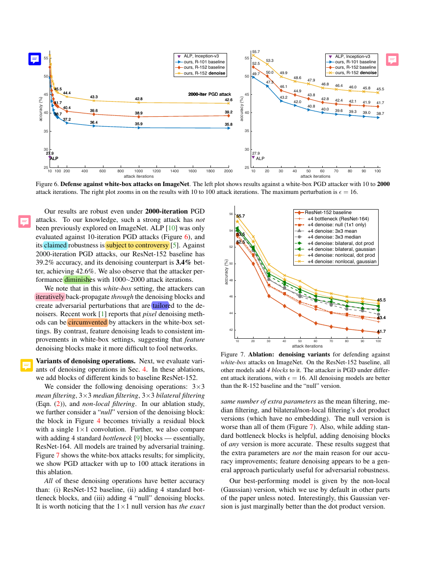
Figure 7 shows the white-box attacks results; for simplicity,
we show PGD attacker with up to 100 attack iterations in
this ablation.
All of these denoising operations have better accuracy
than: (i) ResNet-152 baseline, (ii) adding 4 standard bot-
tleneck blocks, and (iii) adding 4 “null” denoising blocks.
It is worth noticing that the 1×1 null version has the exact
Figure 7. Ablation: denoising variants for defending against
white-box attacks on ImageNet. On the ResNet-152 baseline, all
other models add 4 blocks to it. The attacker is PGD under differ-
ent attack iterations, with � = 16. All denoising models are better
than the R-152 baseline and the “null” version.
same number of extra parameters as the mean filtering, me-
dian filtering, and bilateral/non-local filtering’s dot product
versions (which have no embedding). The null version is
worse than all of them (Figure 7). Also, while adding stan-
dard bottleneck blocks is helpful, adding denoising blocks
of any version is more accurate. These results suggest that
the extra parameters are not the main reason for our accu-
racy improvements; feature denoising appears to be a gen-
eral approach particularly useful for adversarial robustness.
Our best-performing model is given by the non-local
(Gaussian) version, which we use by default in other parts
of the paper unless noted. Interestingly, this Gaussian ver-
sion is just marginally better than the dot product version.
10100200400600800100012001400160018002000attack iterations25303540455055accuracy (%)ALP45.544.443.342.842.641.740.439.638.939.238.737.236.435.935.827.92000-iter PGD attackALP45.544.443.342.842.641.740.439.638.939.238.737.236.435.935.827.92000-iter PGD attackALP, Inception-v3ours, R-101 baselineours, R-152 baselineours, R-152 denoise102030405060708090100attack iterations25303540455055accuracy (%)ALP55.753.349.948.647.946.846.446.045.845.552.550.046.144.943.842.842.442.141.941.749.747.343.242.040.840.039.639.339.038.727.9ALP, Inception-v3ours, R-101 baselineours, R-152 baselineours, R-152 denoise102030405060708090100attack iterations4244464850525456accuracy (%)55.745.553.543.452.541.755.745.553.543.452.541.7ResNet-152 baseline +4 bottleneck (ResNet-164) +4 denoise: null (1x1 only) +4 denoise: 3x3 mean +4 denoise: 3x3 median +4 denoise: bilateral, dot prod +4 denoise: bilateral, gaussian +4 denoise: nonlocal, dot prod +4 denoise: nonlocal, gaussian�
attack iterations
non-local, Gaussian
removing 1×1
removing residual
10
55.7
52.1
NaN
100
45.5
36.8
NaN
Table 1. Ablation: denoising block design for defending against
white-box attacks on ImageNet. Our networks have four (Gaus-
sian) non-local means denoising blocks. We indicate the perfor-
mance of models we were unable to train by “NaN”.
Design decisions of the denoising block. The denoising
block in Figure 4 has a 1×1 layer and a residual connection.
Although both components do not perform denoising, they
are important for the denoising blocks to work well. Next,
we ablate the behavior of the 1×1 and residual connection.
This ablation is in Table 1. We investigate ResNet-152
with four non-local, Gaussian denoising blocks. All models
are all trained by adversarial training. When removing the
1×1 convolution in the denoising block, the accuracy drops
considerably — e.g., decreasing from 45.5% to 36.8% un-
der 100-iteration PGD attacks. On the other hand, removing
the residual connection makes training unstable, and its loss
does not decrease in our adversarial training.
These results suggest that denoising features in itself is
not sufficient. As suppressing noise may also remove use-
ful signals, it appears essential to properly combine the de-
noised features with the input features in denoising blocks.
6.2. Against Black-Box Attacks
Next, we evaluate defending against black-box attacks.
To have an unbiased yet challenging set of attackers, we
study the 5 best attackers of the NIPS 2017 CAAD com-
petition [13], for which code is publicly available. We use
the latest CAAD 2018 evaluation criterion, which we call
“all-or-nothing”: an image is considered correctly classified
only if the model correctly classifies all adversarial versions
of this image created by all attackers. This is a challenging
evaluation scenario for the defender. Following the CAAD
black-box setting, the maximum perturbation for each pixel
is � = 32, which also makes defense more difficult. Note
that our models are trained with � = 16.
Table 2 shows the results of defending against black-box
attacks on ImageNet validation images. To highlight the
difficulty of the new “all-or-nothing” criterion, we find that
the CAAD 2017 winner [15] has only 0.04% accuracy un-
der this criterion. We find that it is mainly vulnerable to two
of the five attackers5,6. If we remove these two attackers,
[15] has 13.4% accuracy in the “all-or-nothing” setting.
With the “all-or-nothing” criterion, our ResNet-152
baseline has 43.1% accuracy against all five attackers.
This number suggests that a successful implementation of
adversarial training is critical for adversarial robustness.
5https://github.com/pfnet-research/nips17-adversarial-attack
6https://github.com/toshi-k/kaggle-nips-2017-adversarial-attack
model
accuracy (%)
CAAD 2017 winner
CAAD 2017 winner, under 3 attackers
ours, R-152 baseline
+4 denoise: null (1×1 only)
+4 denoise: non-local, dot product
+4 denoise: non-local, Gaussian
+all denoise: non-local, Gaussian
0.04
13.4
43.1
44.1
46.2
46.4
49.5
Table 2. Defense against black-box attacks on ImageNet. We
show top-1 classification accuracy on the ImageNet validation set.
The attackers are the 5 best attackers in CAAD 2017. We adopt the
CAAD 2018 “all-or-nothing” criterion for defenders. The 2017
winner has 0.04% accuracy under this strict criterion, and if we
remove the 2 attackers that it is most vulnerable to, it has 13.4%
accuracy under the 3 remaining attackers.
On top of our strong ResNet-152 baseline, adding four
non-local denoising blocks improves the accuracy to 46.4%
(Table 2).
Interestingly, both the Gaussian and dot prod-
uct versions perform similarly (46.4% vs. 46.2%), although
the Gaussian version has more parameters due to its embed-
ding. Furthermore, the null version has 44.1% accuracy —
this is worse than the non-local, dot product version, even
though they have the same number of parameters; this null
version of 1×1 is 1.0% better than the ResNet-152 baseline.
We have also studied the local variants of denoising
blocks, including mean, median, and bilateral filters. They
have 43.6% ∼ 44.4% accuracy in this black-box setting.
Their results are not convincingly better than the null ver-
sion’s results. This suggests that non-local denoising is
more important than local denoising for robustness against
these black-box attackers.
Pushing the envelope. To examine the potential of our
model, we add denoising blocks to all residual blocks (one
denoising block after each residual block) in ResNet-152.
We only study the non-local Gaussian version here. To
make training feasible, we use the sub-sampling trick in
[24]: the feature map of xj in Eqn. (1) is subsampled (by a
2×2 max pooling) when performing the non-local means,
noting that the feature map of xi is still full-sized. We
only use sub-sampling in this case. It achieves a number of
49.5%. This is 6.4% better than the ResNet-152 baseline’s
43.1%, under the black-box setting (Table 2).
CAAD 2018 challenge results. Finally, we report the re-
sults from the latest CAAD 2018 competition. The 2018 de-
fense track adopts the “all-or-nothing” criterion mentioned
above — in this case, every defense entry needs to defend
against 48 unknown attackers submitted to the same chal-
lenge (in contrast to 5 attackers in our above black-box ab-
lation). The test data is a secret, ImageNet-like dataset. The
maximum perturbation for each pixel is � = 32.
�
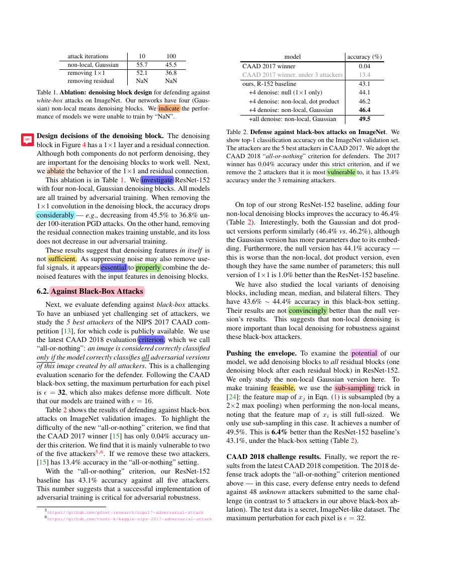
Figure 8. CAAD 2018 results of the adversarial defense track.
The first-place entry is based on our method. We only show the 5
winning submissions here, out of more than 20 submissions.
Figure 8 shows the accuracy of the 5 best entries in the
CAAD 2018 defense track. The winning entry, shown in
the blue bar, was based on our method by using a ResNeXt-
101-32×8 backbone [26] with non-local denoising blocks
added to all residual blocks. This entry only uses single-
It achieves 50.6% accuracy
crop, single-model testing.
against 48 unknown attackers. This is ∼10% absolute (20%
relative) better than the second place’s 40.8% accuracy.
We also reported the white-box performance of this win-
ning entry on ImageNet. Under 10-iteration PGD attacks
and 100-iteration PGD attacks, it achieves 56.0% accuracy
and 40.4% accuracy, respectively. These results are slightly
worse than the robustness of ResNet-152 based models re-
ported in Section 6.1. We note that this white-box robust-
ness comparison is on the system-level as the winning entry
was trained with a slightly different parameter setting.
We emphasize that the CAAD 2018 defense task is very
challenging because of the “all-or-nothing” criterion and
many unknown (potentially new state-of-the-art) attackers.
Actually, except for the two leading teams, all others have
<10% accuracy and many of them have <1% accuracy.
This highlights the significance of our 50.6% accuracy.
6.3. Denoising Blocks in Non-Adversarial Settings
Thus far we have been focusing on denoising blocks
for improving adversarial defense. Because our denoising
blocks are components of the convolutional networks, these
networks can also be trained without adversarial training
for the classification of “clean” images (i.e., the original
ImageNet dataset task). We believe that studying the non-
adversarial setting can help us better understand the behav-
ior of denoising blocks.
In the clean setting,
Table 3 presents the clean image performance of mod-
els that were not adversarially trained. We compare the
baseline R-152, adding standard bottleneck blocks, adding
“null” (1×1) denoising blocks, and adding denoising blocks
of various types.
these denoising
blocks have no obvious advantage over the baseline R-
152, adding standard bottleneck blocks, or adding “null”
denoising blocks. Actually, all results are in the range of
about ±0.2% of the baseline R-152’s result — which have
no significant difference if we also consider the natural vari-
ance between separate training runs of the same model (see
baseline R-152 in Table 3).
model
R-152 baseline
R-152 baseline, run 2
R-152 baseline, run 3
+4 bottleneck (R-164)
+4 denoise: null (1×1 only)
+4 denoise: 3×3 mean filter
+4 denoise: 3×3 median filter
+4 denoise: bilateral, Gaussian
+4 denoise: non-local, Gaussian
accuracy (%)
78.91
+0.05
-0.04
+0.13
+0.15
+0.01
-0.12
+0.15
+0.17
Table 3. Accuracy on clean images in the ImageNet validation set
when trained on clean images. All numbers except the first row are
reported as the accuracy difference comparing with the first R-152
baseline result. For R-152, we run training 3 times independently,
to show the natural random variation of the same architecture. All
denoising models show no significant difference, and are within
±0.2% of the baseline R-152’s result.
We also find that adding non-local denoising blocks to
the shallower ResNet-50 can moderately improve accuracy
by 0.7% in the non-adversarial setting, but doing so on
ResNet-152 has diminishing gain. This, however, is not the
case for the adversarial images.
These results suggest that the denoising blocks could
have special advantages in settings that require adversarial
robustness. This observation matches our intuition that
denoising blocks are designed to reduce feature noise,
which only appears when classifying adversarial images.
Finally, we report that our ResNet-152 baseline with
adversarial training has 62.32% accuracy when tested on
clean images, whereas its counterpart with “clean” train-
ing obtains 78.91%.
For the denoising version (non-
local, Gaussian), the accuracy of an adversarially trained
network is 65.30% on clean images, whereas its cleanly
trained counterpart obtains 79.08%. This tradeoff between
adversarial and clean training has been observed before
(e.g., in [22]); we expect this tradeoff to be the subject of
future research.
7. Conclusion
Motivated by the noisy appearance of feature maps from
adversarial images, we have demonstrated the potential of
feature denoising for improving the adversarial robustness
of convolutional networks. Interestingly, our study suggests
that there are certain architecture designs (viz., denoising
blocks) that are particularly good for adversarial robustness,
even though they do not lead to accuracy improvements
compared to baseline models in “clean” training and testing
scenarios. When combined with adversarial training, these
particular architecture designs may be more appropriate for
modeling the underlying distribution of adversarial images.
We hope our work will encourage researchers to start de-
signing convolutional network architectures that have “in-
nate” adversarial robustness.
0 10203040501st2nd3rd4th5th50.640.8 8.6 3.6 0.6�




 2023年江西萍乡中考道德与法治真题及答案.doc
 2012年重庆南川中考生物真题及答案.doc
 2013年江西师范大学地理学综合及文艺理论基础考研真题.doc
 2020年四川甘孜小升初语文真题及答案I卷.doc
 2020年注册岩土工程师专业基础考试真题及答案.doc
 2023-2024学年福建省厦门市九年级上学期数学月考试题及答案.doc
 2021-2022学年辽宁省沈阳市大东区九年级上学期语文期末试题及答案.doc
 2022-2023学年北京东城区初三第一学期物理期末试卷及答案.doc
 2018上半年江西教师资格初中地理学科知识与教学能力真题及答案.doc
 2012年河北国家公务员申论考试真题及答案-省级.doc
 2020-2021学年江苏省扬州市江都区邵樊片九年级上学期数学第一次质量检测试题及答案.doc
 2022下半年黑龙江教师资格证中学综合素质真题及答案.doc