Clustering by fast search and find of density peaks
Alex Rodriguez and Alessandro Laio
Science
DOI: 10.1126/science.1242072
, 1492 (2014);
344
This copy is for your personal, non-commercial use only.
If you wish to distribute this article to others
colleagues, clients, or customers by
clicking here.
, you can order high-quality copies for your
Permission to republish or repurpose articles or portions of articles
following the guidelines
here.
can be obtained by
The following resources related to this article are available online at
www.sciencemag.org (this information is current as of
June 26, 2014
):
Updated information and services,
version of this article at:
http://www.sciencemag.org/content/344/6191/1492.full.html
including high-resolution figures, can be found in the online
Supporting Online Material
http://www.sciencemag.org/content/suppl/2014/06/25/344.6191.1492.DC1.html
can be found at:
This article
http://www.sciencemag.org/content/344/6191/1492.full.html#ref-list-1
, 1 of which can be accessed free:
cites 14 articles
This article appears in the following
Computers, Mathematics
http://www.sciencemag.org/cgi/collection/comp_math
subject collections:
4
4
4
4
4
4
1
1
1
1
1
1
0
0
0
0
0
0
2
2
2
2
2
2
,
,
,
,
,
,
6
6
6
6
6
6
2
2
2
2
2
2
e
e
e
e
e
e
n
n
n
n
n
n
u
u
u
u
u
u
J
J
J
J
J
J
.
.
.
.
.
.
n
n
n
n
n
n
o
o
o
o
o
o
g
g
g
g
g
g
r
r
r
r
r
r
o
o
o
o
o
o
g
g
g
g
g
g
a
a
a
a
a
a
m
m
m
m
m
m
e
e
e
e
e
e
c
c
c
c
c
c
n
n
n
n
n
n
e
e
e
e
e
e
c
c
c
c
c
c
s
s
s
s
s
s
.
.
.
.
.
.
w
w
w
w
w
w
w
w
w
w
w
w
w
w
w
w
w
w
m
m
m
m
m
m
o
o
o
o
o
o
r
r
r
r
r
r
f
f
f
f
f
f
i
i
i
i
i
i
d
d
d
d
d
d
e
e
e
e
e
e
d
d
d
d
d
d
a
a
a
a
a
a
o
o
o
o
o
o
n
n
n
n
n
n
w
w
w
w
w
w
o
o
o
o
o
o
D
D
D
D
D
D
l
l
l
l
l
l
(print ISSN 0036-8075; online ISSN 1095-9203) is published weekly, except the last week in December, by the
Copyright
Science
American Association for the Advancement of Science, 1200 New York Avenue NW, Washington, DC 20005.
2014 by the American Association for the Advancement of Science; all rights reserved. The title
is a
registered trademark of AAAS.
Science
�
RESEARCH | REPORTS
intrinsic and extrinsic contributions depends on
the sample quality (such as the doping density
and the amount of disorder). Studies of the de-
pendence on temperature and on disorder are
therefore required to better understand the doping
density dependence of the VHE. Furthermore,
a more accurate determination of sH that takes
into account the fringe fields in our Hall bar
device may be needed for a better quantitative
comparison.
optical data on monolayer MoS2. This research was supported by the
Kavli Institute at Cornell for Nanoscale Science and the Cornell
Center for Materials Research [National Science Foundation (NSF)
DMR-1120296]. Additional funding was provided by the Air Force
Office of Scientific Research (FA9550-10-1-0410) and the
Nano-Material Technology Development Program through the National
Research Foundation of Korea funded by the Ministry of Science,
ICT and Future Planning (2012M3A7B4049887). Device fabrication
was performed at the Cornell NanoScale Science and Technology
Facility, a member of the National Nanotechnology Infrastructure
Network, which is supported by NSF (grant ECCS-0335765). K.L.M.
acknowledges support from the NSF Integrative Graduate Education
and Research Traineeship program (DGE-0654193) and the NSF
Graduate Research Fellowship Program (DGE-1144153).
SUPPLEMENTARY MATERIALS
www.sciencemag.org/content/344/6191/1489/suppl/DC1
Materials and Methods
Supplementary Text
Figs. S1 to S10
References (34–37)
24 December 2013; accepted 23 May 2014
10.1126/science.1250140
REFERENCES AND NOTES
1. A. H. Castro Neto, F. Guinea, N. M. R. Peres, K. S. Novoselov,
A. K. Geim, Rev. Mod. Phys. 81, 109–162 (2009).
2. A. Rycerz, J. Tworzydlo, C. W. J. Beenakker, Nat. Phys. 3,
172–175 (2007).
3. A. R. Akhmerov, C. W. J. Beenakker, Phys. Rev. Lett. 98,
157003 (2007).
4. D. Xiao, W. Yao, Q. Niu, Phys. Rev. Lett. 99, 236809 (2007).
5. W. Yao, D. Xiao, Q. Niu, Phys. Rev. B 77, 235406 (2008).
6. D. Xiao, G.-B. Liu, W. Feng, X. Xu, W. Yao, Phys. Rev. Lett. 108,
196802 (2012).
7. Y. J. Zhang, T. Oka, R. Suzuki, J. T. Ye, Y. Iwasa, Science 344,
725–728 (2014).
8. K. F. Mak, C. Lee, J. Hone, J. Shan, T. F. Heinz, Phys. Rev. Lett.
105, 136805 (2010).
9. A. Splendiani et al., Nano Lett. 10, 1271–1275 (2010).
10. T. Cao et al., Nat. Commun. 3, 887 (2012).
11. K. F. Mak, K. He, J. Shan, T. F. Heinz, Nat. Nanotechnol. 7,
494–498 (2012).
12. G. Sallen et al., Phys. Rev. B 86, 081301 (2012).
13. S. Wu et al., Nat. Phys. 9, 149–153 (2013).
14. H. Zeng, J. Dai, W. Yao, D. Xiao, X. Cui, Nat. Nanotechnol. 7,
490–493 (2012).
15. D. Xiao, M.-C. Chang, Q. Niu, Rev. Mod. Phys. 82, 1959–2007
(2010).
16. X. Li, F. Zhang, Q. Niu, Phys. Rev. Lett. 110, 066803 (2013).
17. S. Murakami, N. Nagaosa, S.-C. Zhang, Science 301, 1348–1351
(2003).
18. J. Sinova et al., Phys. Rev. Lett. 92, 126603 (2004).
19. Y. K. Kato, R. C. Myers, A. C. Gossard, D. D. Awschalom,
Science 306, 1910–1913 (2004).
20. J. Wunderlich, B. Kaestner, J. Sinova, T. Jungwirth, Phys. Rev. Lett.
94, 047204 (2005).
21. J. Wunderlich et al., Science 330, 1801–1804 (2010).
22. N. Nagaosa, J. Sinova, S. Onoda, A. H. MacDonald, N. P. Ong,
Rev. Mod. Phys. 82, 1539–1592 (2010).
23. Materials and methods are available as supplementary
materials on Science Online.
24. The skew scattering contribution, which is important only for
high-mobility devices (22), is neglected in MoS2 devices with
relatively low mobility.
25. T. Cheiwchanchamnangij, W. R. L. Lambrecht, Phys. Rev. B 85,
205302 (2012).
26. B. Radisavljevic, A. Radenovic, J. Brivio, V. Giacometti, A. Kis,
Nat. Nanotechnol. 6, 147–150 (2011).
27. L. J. van der Pauw, Philips Techn. Rev. 20, 220–224 (1958).
28. B. W. H. Baugher, H. O. H. Churchill, Y. Yang, P. Jarillo-Herrero,
Nano Lett. 13, 4212–4216 (2013).
29. G. Kioseoglou et al., Appl. Phys. Lett. 101, 221907
(2012).
30. O. Lopez-Sanchez, D. Lembke, M. Kayci, A. Radenovic, A. Kis,
Nat. Nanotechnol. 8, 497–501 (2013).
31. Strictly speaking, a bilayer device with slightly broken inversion
symmetry by the substrate and/or by unintentional doping could
also produce a finite VHE, but these effects are expected to be
much smaller as compared with theVHE in monolayer devices (13).
32. Here, our assumption that only the photoexcited electrons
contribute to the Hall response is reasonable because the
holes are much more vulnerable to traps than are the
electrons, given our highly n-doped device. Unlike the electron
side, the VHE and the SHE become equivalent on the hole side
owing to the spin-valley coupled valence band.
33. H.-A. Engel, B. I. Halperin, E. I. Rashba, Phys. Rev. Lett. 95,
166605 (2005).
ACKNOWLEDGMENTS
We thank D. C. Ralph for his insightful suggestions and J. W. Kevek
for technical support. We also thank J. Shan for many fruitful
discussions and Y. You for private communications regarding the
MACHINE LEARNING
Clustering by fast search and find of
density peaks
Alex Rodriguez and Alessandro Laio
Cluster analysis is aimed at classifying elements into categories on the basis of their
similarity. Its applications range from astronomy to bioinformatics, bibliometrics, and pattern
recognition. We propose an approach based on the idea that cluster centers are characterized
by a higher density than their neighbors and by a relatively large distance from points with
higher densities. This idea forms the basis of a clustering procedure in which the number of
clusters arises intuitively, outliers are automatically spotted and excluded from the analysis, and
clusters are recognized regardless of their shape and of the dimensionality of the space in which
they are embedded. We demonstrate the power of the algorithm on several test cases.
C lustering algorithms attempt to classify
elements into categories, or clusters, on
the basis of their similarity. Several dif-
ferent clustering strategies have been pro-
posed (1), but no consensus has been reached
even on the definition of a cluster. In K-means (2)
and K-medoids (3) methods, clusters are groups
of data characterized by a small distance to the
cluster center. An objective function, typically the
sum of the distance to a set of putative cluster
centers, is optimized (3–6) until the best cluster
centers candidates are found. However, because
a data point is always assigned to the nearest
center, these approaches are not able to detect
nonspherical clusters (7). In distribution-based al-
gorithms, one attempts to reproduce the observed
realization of data points as a mix of predefined
probability distribution functions (8); the accuracy
of such methods depends on the capability of the
trial probability to represent the data.
Clusters with an arbitrary shape are easily
detected by approaches based on the local den-
sity of data points. In density-based spatial clus-
tering of applications with noise (DBSCAN) (9),
one chooses a density threshold, discards as noise
the points in regions with densities lower than
this threshold, and assigns to different clusters
disconnected regions of high density. However,
choosing an appropriate threshold can be non-
trivial, a drawback not present in the mean-shift
clustering method (10, 11). There a cluster is de-
fined as a set of points that converge to the same
local maximum of the density distribution func-
SISSA (Scuola Internazionale Superiore di Studi Avanzati),
via Bonomea 265, I-34136 Trieste, Italy.
E-mail: laio@sissa.it (A.L.); alexrod@sissa.it (A.R.)
tion. This method allows the finding of nonspheri-
cal clusters but works only for data defined by a
set of coordinates and is computationally costly.
Here, we propose an alternative approach.
Similar to the K-medoids method, it has its
basis only in the distance between data points.
Like DBSCAN and the mean-shift method, it is
able to detect nonspherical clusters and to auto-
matically find the correct number of clusters.
The cluster centers are defined, as in the mean-
shift method, as local maxima in the density of
data points. However, unlike the mean-shift meth-
od, our procedure does not require embedding
the data in a vector space and maximizing ex-
plicitly the density field for each data point.
The algorithm has its basis in the assumptions
that cluster centers are surrounded by neighbors
with lower local density and that they are at a
relatively large distance from any points with a
higher local density. For each data point i, we
compute two quantities: its local density ri and
its distance di from points of higher density. Both
these quantities depend only on the distances dij
between data points, which are assumed to satis-
fy the triangular inequality. The local density ri
of data point i is defined as
ri ¼ ∑
j
cðdij − dcÞ
ð1Þ
where cðxÞ ¼ 1 if x < 0 and cðxÞ ¼ 0 otherwise,
and dc is a cutoff distance. Basically, ri is equal to
the number of points that are closer than dc to
point i. The algorithm is sensitive only to the rel-
ative magnitude of ri in different points, implying
that, for large data sets, the results of the analysis
are robust with respect to the choice of dc.
1492
27 JUNE 2014 VOL 344 ISSUE 6191
sciencemag.org SCIENCE
�
di is measured by computing the minimum
distance between the point i and any other
point with higher density:
di ¼ min
ðdijÞ
ð2Þ
j:rj >ri
RESEARCH | REPORTS
For the point with highest density, we con-
ventionally take di ¼ maxjðdijÞ. Note that di is
much larger than the typical nearest neighbor
distance only for points that are local or global
maxima in the density. Thus, cluster centers are
recognized as points for which the value of di is
anomalously large.
This observation, which is the core of the
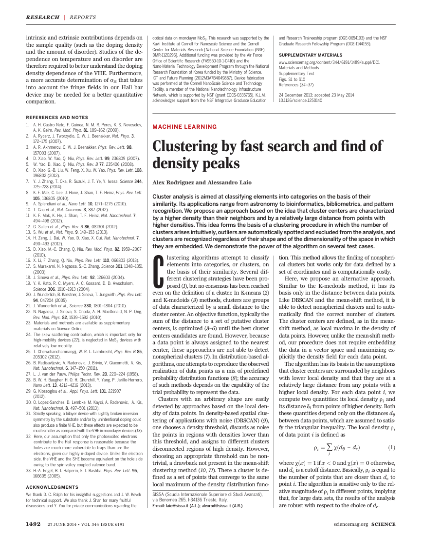
algorithm, is illustrated by the simple example
in Fig. 1. Figure 1A shows 28 points embedded
Fig. 1. The algorithm in two dimensions. (A) Point distribution. Data points are ranked in order of decreasing density. (B) Decision graph for the data in
(A). Different colors correspond to different clusters.
0.5
0.4
0.3
0.2
0.1
0.0
0.0100
0.0075
0.0050
0.0025
0
40
80
120
160
0.4
0.3
0.2
0.1
0.0
0
150
300
450
0.0000
0
2000
4000
6000
Number of points
8000
10,000
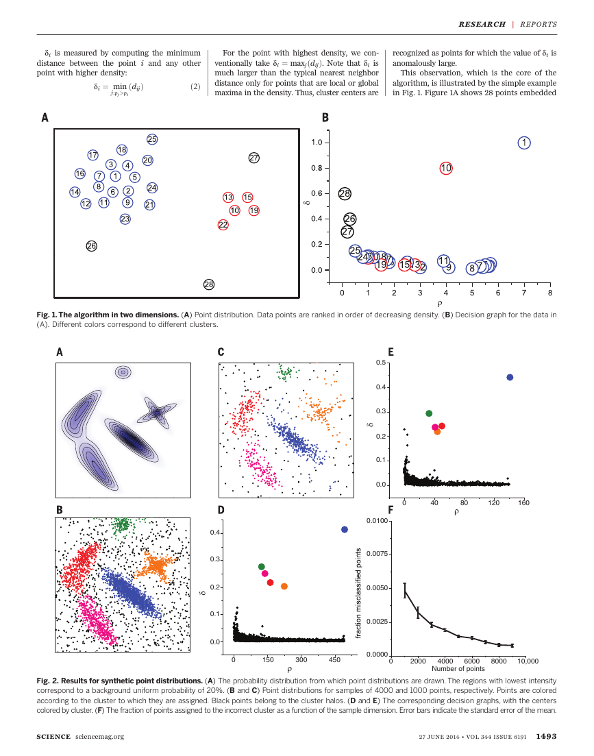
Fig. 2. Results for synthetic point distributions. (A) The probability distribution from which point distributions are drawn. The regions with lowest intensity
correspond to a background uniform probability of 20%. (B and C) Point distributions for samples of 4000 and 1000 points, respectively. Points are colored
according to the cluster to which they are assigned. Black points belong to the cluster halos. (D and E) The corresponding decision graphs, with the centers
colored by cluster. (F) The fraction of points assigned to the incorrect cluster as a function of the sample dimension. Error bars indicate the standard error of the mean.
SCIENCE sciencemag.org
27 JUNE 2014 VOL 344 ISSUE 6191
1493
�
RESEARCH | REPORTS
in a two-dimensional space. We find that the
density maxima are at points 1 and 10, which we
identify as cluster centers. Figure 1B shows the
plot of di as a function of ri for each point; we
will call this representation the decision graph.
The value of d for points 9 and 10, with similar
values of r, is very different: Point 9 belongs to
the cluster of point 1, and several other points
with a higher r are very close to it, whereas the
nearest neighbor of higher density of point 10
belongs to another cluster. Hence, as anticipated,
the only points of high d and relatively high r are
the cluster centers. Points 26, 27, and 28 have a
relatively high d and a low r because they are
isolated; they can be considered as clusters com-
posed of a single point, namely, outliers.
After the cluster centers have been found, each
remaining point is assigned to the same cluster
as its nearest neighbor of higher density. The clus-
ter assignment is performed in a single step, in
contrast with other clustering algorithms where
an objective function is optimized iteratively (2, 8).
In cluster analysis, it is often useful to measure
quantitatively the reliability of an assignment. In
approaches based on the optimization of a func-
tion (2, 8), its value at convergence is also a
natural quality measure. In methods like DBSCAN
(9), one considers reliable points with density
values above a threshold, which can lead to low-
density clusters, such as those in Fig. 2E, being
classified as noise. In our algorithm, we do not
introduce a noise-signal cutoff. Instead, we first
find for each cluster a border region, defined as
the set of points assigned to that cluster but being
within a distance dc from data points belonging to
other clusters. We then find, for each cluster, the
point of highest density within its border region.
We denote its density by rb. The points of the
cluster whose density is higher than rb are consid-
ered part of the cluster core (robust assignation).
The others are considered part of the cluster halo
(suitable to be considered as noise).
In order to benchmark our procedure, let us
first consider the test case in Fig. 2. The data
points are drawn from a probability distribution
with nonspherical and strongly overlapping peaks
(Fig. 2A); the probability values corresponding
to the maxima differ by almost an order of mag-
nitude. In Fig. 2, B and C, 4000 and 1000 points,
respectively, are drawn from the distribution in
Fig. 2A. In the corresponding decision graphs
(Fig. 2, D and E), we observe only five points with
a large value of d and a sizeable density. These
points are represented in the graphs as large solid
circles and correspond to cluster centers. After
the centers have been selected, each point is
assigned either to a cluster or to the halo. The
algorithm captures the position and shape of
the probability peaks, even those correspond-
ing to very different densities (blue and light
green points in Fig. 2C) and nonspherical peaks.
Moreover, points assigned to the halo correspond
to regions that by visual inspection of the prob-
ability distribution in Fig. 2A would not be
assigned to any peak.
To demonstrate the robustness of the proce-
dure more quantitatively, we performed the analy-
sis by drawing 10,000 points from the distribution
in Fig. 2A, considering as a reference the cluster
assignment obtained on that sample. We then
obtained reduced samples by retaining only a
fraction of points and performed cluster assign-
ment for each reduced sample independently.
Figure 2F shows, as a function of the size of the
reduced sample, the fraction of points assigned to
a cluster different than the one they were as-
signed to in the reference case. The fraction of
misclassified points remains well below 1% even
for small samples containing 1000 points.
Varying dc for the data in Fig. 2B produced
mutually consistent results (fig. S1). As a rule of
thumb, one can choose dc so that the average
number of neighbors is around 1 to 2% of the
total number of points in the data set. For data
Fig. 3. Results for test cases in the literature. Synthetic point distributions from (12) (A), (13) (B), (14) (C), and (15) (D).
1494
27 JUNE 2014 VOL 344 ISSUE 6191
sciencemag.org SCIENCE
�
sets composed by a small number of points, ri
might be affected by large statistical errors. In
these cases, it might be useful to estimate the
density by more accurate measures (10, 11).
Next, we benchmarked the algorithm on the
test cases presented in Fig. 3. For computing the
density for cases with few points, we adopted
the exponential kernel described in (11). In Fig.
3A, we consider a data set from (12), obtaining
results comparable to those of the original ar-
ticle, where it was shown that other commonly
used methods fail. In Fig. 3B, we consider an
example with 15 clusters with high overlap in
data distribution taken from (13); our algorithm
successfully determines the cluster structure of
the data set. In Fig. 3C, we consider the test case
for the FLAME (fuzzy clustering by local approx-
imation of membership) approach (14), with re-
sults comparable to the original method. In the
data set originally introduced to illustrate the
performance of path-based spectral clustering
(15) shown in Fig. 4D, our algorithm correctly
finds the three clusters without the need of gen-
erating a connectivity graph. As comparison, in
figs. S3 and S4 we show the cluster assignations
obtained by K-means (2) for these four test cases
and for the example in Fig. 2. Even if the K-means
optimization is performed with use of the correct
value of K, the assignations are, in most of the
cases, not compliant with visual intuition.
The method is robust with respect to changes
in the metric that do not significantly affect the
distances below dc, that is, that keep the density
estimator in Eq. 1 unchanged. Clearly, the distance
in Eq. 2 will be affected by such a change of metric,
but it is easy to realize that the structure of the
decision graph (in particular, the number of data
points with a large value of d) is a consequence of
the ranking of the density values, not of the actual
distance between far away points. Examples dem-
onstrating this statement are shown in fig. S5.
Our approach only requires measuring (or
computing) the distance between all the pairs
of data points and does not require parame-
terizing a probability distribution (8) or a mul-
tidimensional density function (10). Therefore,
its performance is not affected by the intrinsic
dimensionality of the space in which the data
points are embedded. We verified that, in a test
case with 16 clusters in 256 dimensions (16), the
algorithm finds the number of clusters and as-
signs the points correctly (fig. S6). For a data set
with 210 measurements of seven x-ray features
for three types of wheat seeds from (17), the al-
gorithm correctly predicts the existence of three
clusters and classifies correctly 97% of the points
assigned to the cluster cores (figs. S7 and S8).
We also applied the approach to the Olivetti
Face Database (18), a widespread benchmark for
machine learning algorithms, with the aim of
RESEARCH | REPORTS
identifying, without any previous training, the
number of subjects in the database. This data set
poses a serious challenge to our approach be-
cause the “ideal” number of clusters (namely of
distinct subjects) is comparable with the num-
ber of elements in the data set (namely of different
images, 10 for each subject). This makes a reliable
estimate of the densities difficult. The similarity
between two images was computed by following
(19). The density is estimated by a Gaussian ker-
nel (11) with variance dc ¼ 0:07. For such a small
set, the density estimator is unavoidably affected
by large statistical errors; thus, we assign images
to a cluster following a slightly more restrictive
criterion than in the preceding examples. An im-
age is assigned to the same cluster of its nearest
image with higher density only if their distance
is smaller than dc. As a consequence, the images
further than dc from any other image of higher
density remain unassigned. In Fig. 4, we show
the results of an analysis performed for the first
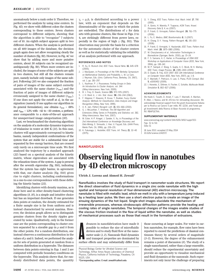
100 images in the data set. The decision graph
(Fig. 4A) shows the presence of several distinct
density maxima. Unlike in other examples, their
exact number is not clear, a consequence of the
sparsity of the data points. A hint for choosing
the number of centers is provided by the plot of
gi ¼ ridi sorted in decreasing order (Fig. 4B).
This graph shows that this quantity, that is by
definition large for cluster centers, starts growing
Fig. 4. Cluster analysis of the Olivetti Face Database. (A) The decision
graph for the first hundred images in the database (18). (B) The value of
γi ¼ ridi in decreasing order for the data in (A). (C) The performance of
the algorithm in recognizing subjects in the full database as a function
of the number of clusters: number of subjects recognized as individuals
(black line), number of clusters that include more than one subject (red
line), number of subjects split in more than one cluster (green), and num-
ber of images assigned to a cluster divided by 10 (purple). (D) Pictorial
representation of the cluster assignations for the first 100 images.
Faces with the same color belong to the same cluster, whereas gray
images are not assigned to any cluster. Cluster centers are labeled with
white circles.
SCIENCE sciencemag.org
27 JUNE 2014 VOL 344 ISSUE 6191
1495
�
RESEARCH | REPORTS
anomalously below a rank order 9. Therefore, we
performed the analysis by using nine centers. In
Fig. 4D, we show with different colors the clusters
corresponding to these centers. Seven clusters
correspond to different subjects, showing that
the algorithm is able to “recognize” 7 subjects
out of 10. An eighth subject appears split in two
different clusters. When the analysis is performed
on all 400 images of the database, the decision
graph again does not allow recognizing clearly the
number of clusters (fig. S9). However, in Fig. 4C we
show that by adding more and more putative
centers, about 30 subjects can be recognized un-
ambiguously (fig. S9). When more centers are in-
cluded, the images of some of the subjects are split
in two clusters, but still all the clusters remain
pure, namely include only images of the same sub-
ject. Following (20) we also computed the fraction
of pairs of images of the same subject correctly
associated with the same cluster (rtrue) and the
fraction of pairs of images of different subjects
erroneously assigned to the same cluster (rfalse).
If one does not apply the cutoff at dc in the as-
signation (namely if one applies our algorithm in
its general formulation), one obtains rtrue ~ 68%
and rfalse ~ 1.2% with ~42 to ~50 centers, a perform-
ance comparable to a state-of-the-art approach
for unsupervised image categorization (20).
Last, we benchmarked the clustering algorithm
on the analysis of a molecular dynamics trajectory
of trialanine in water at 300 K (21). In this case,
clusters will approximately correspond to kinetic
basins, namely independent conformations of the
system that are stable for a substantial time and
separated by free energy barriers, that are crossed
only rarely on a microscopic time scale. We first
analyzed the trajectory by a standard approach
(22) based on a spectral analysis of the kinetic
matrix, whose eigenvalues are associated with
the relaxation times of the system. A gap is present
after the seventh eigenvalue (fig. S10), indicating
that the system has eight basins; in agreement
with that, our cluster analysis (fig. S10) gives
rise to eight clusters, including conformations
in a one-to-one correspondence with those defin-
ing the kinetic basins (22).
Identifying clusters with density maxima, as is
done here and in other density-based clustering
algorithms (9, 10), is a simple and intuitive choice
but has an important drawback. If one generates
data points at random, the density estimated for
a finite sample size is far from uniform and is
instead characterized by several maxima. How-
ever, the decision graph allows us to distinguish
genuine clusters from the density ripples gen-
erated by noise. Qualitatively, only in the former
case are the points corresponding to cluster cen-
ters separated by a sizeable gap in r and d from
the other points. For a random distribution, one
instead observes a continuous distribution in the
values of r and d. Indeed, we performed the analy-
sis for sets of points generated at random from a
uniform distribution in a hypercube. The distances
between data points entering in Eqs. 1 and 2 are
computed with periodic boundary conditions on
the hypercube. This analysis shows that, for ran-
domly distributed data points, the quantity
1496
27 JUNE 2014 VOL 344 ISSUE 6191
gi ¼ ridi is distributed according to a power
law, with an exponent that depends on the
dimensionality of the space in which the points
are embedded. The distributions of g for data
sets with genuine clusters, like those in Figs. 2 to
4, are strikingly different from power laws, es-
pecially in the region of high g (fig. S11). This
observation may provide the basis for a criterion
for the automatic choice of the cluster centers
as well as for statistically validating the reliability
of an analysis performed with our approach.
REFERENCES AND NOTES
1. R. Xu, D. Wunsch 2nd, IEEE Trans. Neural Netw. 16, 645–678
2.
(2005).
J. MacQueen, in Proceedings of the Fifth Berkeley Symposium
on Mathematical Statistics and Probability, L. M. Le Cam,
J. Neyman, Eds. (Univ. California Press, Berkeley, CA, 1967),
vol. 1, pp. 281–297.
3. L. Kaufman, P. J. Rousseeuw, Finding Groups in Data:
An Introduction to Cluster Analysis, vol. 344
(Wiley-Interscience, New York, 2009).
4. B. J. Frey, D. Dueck, Science 315, 972–976 (2007).
5.
6. F. Höppner, F. Klawonn, R. Kruse, T. Runkler, Fuzzy Cluster
J. H. Ward Jr., J. Am. Stat. Assoc. 58, 236–244 (1963).
Analysis: Methods for Classification, Data Analysis and Image
Recognition (Wiley, New York, 1999).
7. A. K. Jain, Pattern Recognit. Lett. 31, 651–666 (2010).
8. G. J. McLachlan, T. Krishnan, The EM Algorithm and
Extensions (Wiley Series in Probability and Statistics vol. 382,
Wiley-Interscience, New York, 2007).
9. M. Ester, H.-P. Kriegel, J. Sander, X. Xu, in Proceedings of the
2nd International Conference on Knowledge Discovery and
Data Mining, E. Simoudis, J. Han, U. Fayyad, Eds. (AAAI Press,
Menlo Park, CA, 1996), pp. 226–231.
10. K. Fukunaga, L. Hostetler, IEEE Trans. Inf. Theory 21, 32–40
(1975).
11. Y. Cheng, IEEE Trans. Pattern Anal. Mach. Intell. 17, 790
(1995).
12. A. Gionis, H. Mannila, P. Tsaparas, ACM Trans. Knowl.
Discovery Data 1, 4, es (2007).
13. P. Fränti, O. Virmajoki, Pattern Recognit. 39, 761–775
(2006).
14. L. Fu, E. Medico, BMC Bioinformatics 8, 3 (2007).
15. H. Chang, D.-Y. Yeung, Pattern Recognit. 41, 191–203
(2008).
16. P. Fränti, O. Virmajoki, V. Hautamäki, IEEE Trans. Pattern Anal.
Mach. Intell. 28, 1875–1881 (2006).
17. M. Charytanowicz et al., Information Technologies in
Biomedicine (Springer, Berlin, 2010), pp. 15–24.
18. F. S. Samaria, A. C. Harter, in Proceedings of 1994 IEEE
Workshop on Applications of Computer Vision (IEEE, New York,
1994), pp. 138–142.
19. M. P. Sampat, Z. Wang, S. Gupta, A. C. Bovik, M. K. Markey,
IEEE Trans. Image Process. 18, 2385–2401 (2009).
20. D. Dueck, B. Frey, ICCV 2007. IEEE 11th International Conference
on Computer Vision (IEEE, New York, 2007), pp. 1–8.
21. F. Marinelli, F. Pietrucci, A. Laio, S. Piana, PLOS Comput. Biol.
5, e1000452 (2009).
22. I. Horenko, E. Dittmer, A. Fischer, C. Schütte, Multiscale Model.
Simulation 5, 802–827 (2006).
ACKNOWLEDGMENTS
We thank E. Tosatti, D. Amati, F. Laio, F. Marinelli, A. Maritan,
R. Allen, J. Nasica, and M. d’Errico for stimulating discussion. We
acknowledge financial support from the grant Associazione Italiana
per la Ricerca sul Cancro 5 per mille, Rif. 12214, and Fondo per
gli Investimenti della Ricerca di Base–Accordo di programma,
Rif. RBAP11ETKA.
SUPPLEMENTARY MATERIALS
www.sciencemag.org/content/344/6191/1492/suppl/DC1
Figs. S1 to S11
Data S1
18 June 2013; accepted 23 May 2014
10.1126/science.1242072
NANOFLUIDICS
Observing liquid flow in nanotubes
by 4D electron microscopy
Ulrich J. Lorenz and Ahmed H. Zewail*
Nanofluidics involves the study of fluid transport in nanometer-scale structures. We report
the direct observation of fluid dynamics in a single zinc oxide nanotube with the high
spatial and temporal resolution of four-dimensional (4D) electron microscopy. The
nanotube is filled with metallic lead, which we melt in situ with a temperature jump induced
by a heating laser pulse. We then use a short electron pulse to create an image of the
ensuing dynamics of the hot liquid. Single-shot images elucidate the mechanism of
irreversible processes, whereas stroboscopic diffraction patterns provide the heating and
cooling rates of single nanotubes. The temporal changes of the images enable studies of
the viscous friction involved in the flow of liquid within the nanotube, as well as studies
of mechanical processes such as those that result in the formation of extrusions.
those occurring at larger scales. For water in car-
bon nanotubes, for example, flow rates have been
reported to exceed the predictions of classical con-
tinuum theory by several orders of magnitude
(3–5). However, the degree of the enhancement
remains a point of discussion (6). The study of a
single nanochannel, rather than a large ensemble,
should reduce the experimental uncertainty and
provide an opportunity to visualize mechanical
and fluid dynamics at the nanoscale. Such exper-
iments not only incur the challenge of preparing
sciencemag.org SCIENCE
A dvances in nanofabrication have made it
possible to reduce the size of microfluidic
devices and to study fluid flow at the nano-
meter scale (1, 2). Nanoscale fluid dynamics
and transport properties are dominated by
surface effects and may substantially differ from
Physical Biology Center for Ultrafast Science and
Technology, Arthur Amos Noyes Laboratory of Chemical
Physics, California Institute of Technology, Pasadena, CA
91125, USA.
*Corresponding author. E-mail: zewail@caltech.edu
�





 2023年江西萍乡中考道德与法治真题及答案.doc
 2012年重庆南川中考生物真题及答案.doc
 2013年江西师范大学地理学综合及文艺理论基础考研真题.doc
 2020年四川甘孜小升初语文真题及答案I卷.doc
 2020年注册岩土工程师专业基础考试真题及答案.doc
 2023-2024学年福建省厦门市九年级上学期数学月考试题及答案.doc
 2021-2022学年辽宁省沈阳市大东区九年级上学期语文期末试题及答案.doc
 2022-2023学年北京东城区初三第一学期物理期末试卷及答案.doc
 2018上半年江西教师资格初中地理学科知识与教学能力真题及答案.doc
 2012年河北国家公务员申论考试真题及答案-省级.doc
 2020-2021学年江苏省扬州市江都区邵樊片九年级上学期数学第一次质量检测试题及答案.doc
 2022下半年黑龙江教师资格证中学综合素质真题及答案.doc