logo资料库

TraMineR-Users-Guide(R语言文本挖掘包TraMineR).pdf

第1页 / 共129页
第2页 / 共129页
第3页 / 共129页
第4页 / 共129页
第5页 / 共129页
第6页 / 共129页
第7页 / 共129页
第8页 / 共129页
资料共129页,剩余部分请下载后查看
Introduction
Aims and features of the TraMineR package
A short example to begin with
State sequence analysis
Event sequence analysis
The TraMineR package
Loading, using and getting help
Data sets included in the TraMineR package
The actcal data set
The biofam data set
The mvad data set
Other data sets borrowed from the literature
Performance and memory usage
Definition and representation of longitudinal data formats
Ontology
States and events
Single or multichannel
Time reference: Internal and external clocks
One or several rows per individual
Ontology
Longitudinal data representations
The `states-sequence' (STS) format
The `state-permanence-sequence' (SPS) format
The vertical `time-stamped-event' (TSE) format
The spell (SPELL) format
The `person-period' format
The `shifted-replicated-sequence' format (SRS)
Definition and properties of categorical sequences
Categorical sequences
Time axis
Subsequences
Importing and handling longitudinal data with TraMineR
Importing data sets into R
Reading data from other statistical packages
Reading data from text files
Data storage in R
Compressed and extended format
Converting between formats
Converting between compressed and extended formats
The seqformat function
Creating state sequence objects
Creating a state sequence object
Creating a sequence object from SPS-formatted data
Creating a sequence object from SPELL-formatted data
Attributes of sequence objects
State codes
Alphabet
Color palette
State labels
Starting time
Summarizing sequence objects
Indexing and printing sequence objects
Truncations, gaps and missing values
Introduction
Handling the different kinds of missing values
Describing and visualizing state sequences
General principle of TraMineR sequence plots
Color palette representing the states
Plotting the legend separately
Describing and visualizing sequence data sets
List of states present in sequence data
State distribution
Sequence frequencies
Transition rates
Mean time spent in each state
Describing and visualizing individual sequences
Visualizing individual sequences
Finding sequences with a given subsequence
Sequence characteristics and associated measures
Basic sequence characteristics
Sequence length
Distinct states and durations
Summarizing the DSS
Number of subsequences
Number of transitions
Summarizing state durations
Variance of the state durations
Cumulated state durations
Within sequence entropy
Composite measures of sequences complexity
Sequence turbulence
Measuring similarities and distances between sequences
Number of matching positions
Longest Common Prefix (LCP) distances
LCP based metric
Computing LCP distances
Longest Common Subsequence (LCS) distances
LCS based metric
Computing LCS distances
LCS distances with internal gaps
Optimal matching (OM) distances
The insertion/deletion cost
The substitution-cost matrix
Generating optimal matching distances
LCS distance as a special case of OM distance
Optimal matching with internal gaps
Clustering distance matrices
Analysing event sequences
Creating event sequences
Searching for frequent event subsequences
Plotting the results
Time constraints
Identifying discriminant event subsequences
Plotting the results
More advanced topics and utilities
Looking after specific subsequences
Counting the number of occurrence in each event sequence
Selecting event subsequences
Duration of event sequences
Installing and using R
Obtaining and installing R
R basics
Data manipulation in R
Creating and printing objects
Vectors
Data frames, matrices and lists
Accessing and extracting data
R libraries
Some other useful functions
The apply function
The table function
Creating and saving graphics
Performance and memory usage
Information about TraMineR content
Bibliography
Mining sequence data in R with the TraMineR package: A user’s guide1 (for version 1.8) Alexis Gabadinho, Gilbert Ritschard, Matthias Studer and Nicolas S. M¨uller Department of Econometrics and Laboratory of Demography University of Geneva, Switzerland http://mephisto.unige.ch/traminer/ March 18, 2011 1This work is part of the research project “Mining event histories: Towards new insights on personal Swiss life courses” supported by the Swiss National Science Foundation under grants FN-100012-113998 and FN-100015-122230.
2 Acknowledgments: TraMineR was mainly developed on a Ubuntu/Linux system with several open-source free tools and programs, including of course R and the LATEX language used to write this manual. We would like to thank all the contributors to those free softwares. We also would like to thank Cees Elzinga for providing us the code of his CHESA software for sequence analysis, which was helpful to program some of the metrics he introduced to compute distances between sequences. Thanks also to the participants of the Research Seminar in Statistics for the Social Sciences and Demography in Geneva as well as to the participants of the Workshop on Sequential Data Analysis held in Lund, Sweden, May 8-9 2008, for their useful remarks and for β-testing earlier versions of the package. Thanks also to the Swiss Household Panel who authorized us to use a sample of their data, and to D. McVicar and M. Anyadike-Danes for the permission regarding the mvad data set they used in an article of the Journal of the Royal Statistical Society. Those data sets are included in the TraMineR package and are used for illustrating this user’s guide. Reporting bugs: We have indeed carefully tested the package. Nevertheless, we cannot exclude that there remain programming errors and encourage you to report any bugs you may encounter to the package maintainer who is presently alexis.gabadinho@unige.ch. You will thus contribute to improve the package. Referencing TraMineR: Thank you for citing this User’s guide, i.e. Gabadinho, A., G. Ritschard, M. Studer and N. S. M¨uller Mining sequence data in R with the TraMineR package: A user’s guide University of Geneva, 2010. (http://mephisto.unige.ch/traminer) when presenting analyses realized with the help of TraMineR.
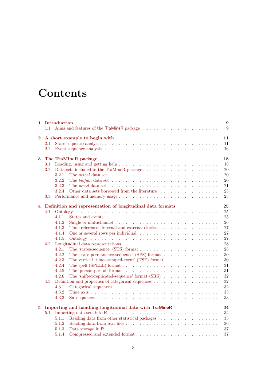
Contents 1 Introduction 1.1 Aims and features of the TraMineR package . . . . . . . . . . . . . . . . . . . . . . 2 A short example to begin with 2.1 State sequence analysis . . . . . . . . . . . . . . . . . . . . . . . . . . . . . . . . . . 2.2 Event sequence analysis . . . . . . . . . . . . . . . . . . . . . . . . . . . . . . . . . 3 The TraMineR package 3.1 Loading, using and getting help . . . . . . . . . . . . . . . . . . . . . . . . . . . . . 3.2 Data sets included in the TraMineR package . . . . . . . . . . . . . . . . . . . . . . 3.2.1 The actcal data set . . . . . . . . . . . . . . . . . . . . . . . . . . . . . . . 3.2.2 The biofam data set . . . . . . . . . . . . . . . . . . . . . . . . . . . . . . . 3.2.3 The mvad data set . . . . . . . . . . . . . . . . . . . . . . . . . . . . . . . . 3.2.4 Other data sets borrowed from the literature . . . . . . . . . . . . . . . . . 3.3 Performance and memory usage . . . . . . . . . . . . . . . . . . . . . . . . . . . . . 4 Definition and representation of longitudinal data formats 4.2 Longitudinal data representations 4.1 Ontology . . . . . . . . . . . . . . . . . . . . . . . . . . . . . . . . . . . . . . . . . States and events . . . . . . . . . . . . . . . . . . . . . . . . . . . . . . . . . 4.1.1 4.1.2 . . . . . . . . . . . . . . . . . . . . . . . . . . . . . . Single or multichannel 4.1.3 Time reference: Internal and external clocks . . . . . . . . . . . . . . . . . . 4.1.4 One or several rows per individual . . . . . . . . . . . . . . . . . . . . . . . 4.1.5 Ontology . . . . . . . . . . . . . . . . . . . . . . . . . . . . . . . . . . . . . . . . . . . . . . . . . . . . . . . . . . . . . . . . 4.2.1 The ‘states-sequence’ (STS) format . . . . . . . . . . . . . . . . . . . . . . . 4.2.2 The ‘state-permanence-sequence’ (SPS) format . . . . . . . . . . . . . . . . 4.2.3 The vertical ‘time-stamped-event’ (TSE) format . . . . . . . . . . . . . . . 4.2.4 The spell (SPELL) format . . . . . . . . . . . . . . . . . . . . . . . . . . . . 4.2.5 The ‘person-period’ format . . . . . . . . . . . . . . . . . . . . . . . . . . . 4.2.6 The ‘shifted-replicated-sequence’ format (SRS) . . . . . . . . . . . . . . . . 4.3 Definition and properties of categorical sequences . . . . . . . . . . . . . . . . . . . 4.3.1 Categorical sequences . . . . . . . . . . . . . . . . . . . . . . . . . . . . . . 4.3.2 Time axis . . . . . . . . . . . . . . . . . . . . . . . . . . . . . . . . . . . . . 4.3.3 Subsequences . . . . . . . . . . . . . . . . . . . . . . . . . . . . . . . . . . . 5 Importing and handling longitudinal data with TraMineR 5.1 Importing data sets into R . . . . . . . . . . . . . . . . . . . . . . . . . . . . . . . . 5.1.1 Reading data from other statistical packages . . . . . . . . . . . . . . . . . 5.1.2 Reading data from text files . . . . . . . . . . . . . . . . . . . . . . . . . . . 5.1.3 Data storage in R . . . . . . . . . . . . . . . . . . . . . . . . . . . . . . . . . 5.1.4 Compressed and extended format . . . . . . . . . . . . . . . . . . . . . . . . 9 9 11 11 16 18 18 20 20 20 21 23 23 25 25 25 26 27 27 27 28 28 30 30 31 31 32 32 32 33 33 34 34 35 36 37 37 3
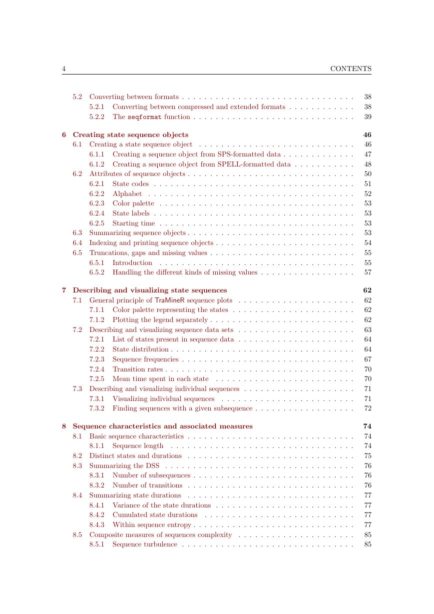
4 CONTENTS 5.2 Converting between formats . . . . . . . . . . . . . . . . . . . . . . . . . . . . . . . 5.2.1 Converting between compressed and extended formats . . . . . . . . . . . . 5.2.2 The seqformat function . . . . . . . . . . . . . . . . . . . . . . . . . . . . . 6 Creating state sequence objects 6.1 Creating a state sequence object . . . . . . . . . . . . . . . . . . . . . . . . . . . . 6.1.1 Creating a sequence object from SPS-formatted data . . . . . . . . . . . . . 6.1.2 Creating a sequence object from SPELL-formatted data . . . . . . . . . . . 6.2 Attributes of sequence objects . . . . . . . . . . . . . . . . . . . . . . . . . . . . . . State codes . . . . . . . . . . . . . . . . . . . . . . . . . . . . . . . . . . . . 6.2.1 6.2.2 Alphabet . . . . . . . . . . . . . . . . . . . . . . . . . . . . . . . . . . . . . 6.2.3 Color palette . . . . . . . . . . . . . . . . . . . . . . . . . . . . . . . . . . . State labels . . . . . . . . . . . . . . . . . . . . . . . . . . . . . . . . . . . . 6.2.4 6.2.5 Starting time . . . . . . . . . . . . . . . . . . . . . . . . . . . . . . . . . . . 6.3 Summarizing sequence objects . . . . . . . . . . . . . . . . . . . . . . . . . . . . . . 6.4 Indexing and printing sequence objects . . . . . . . . . . . . . . . . . . . . . . . . . 6.5 Truncations, gaps and missing values . . . . . . . . . . . . . . . . . . . . . . . . . . 6.5.1 Introduction . . . . . . . . . . . . . . . . . . . . . . . . . . . . . . . . . . . 6.5.2 Handling the different kinds of missing values . . . . . . . . . . . . . . . . . 7 Describing and visualizing state sequences 7.1 General principle of TraMineR sequence plots . . . . . . . . . . . . . . . . . . . . . 7.1.1 Color palette representing the states . . . . . . . . . . . . . . . . . . . . . . 7.1.2 Plotting the legend separately . . . . . . . . . . . . . . . . . . . . . . . . . . 7.2 Describing and visualizing sequence data sets . . . . . . . . . . . . . . . . . . . . . 7.2.1 List of states present in sequence data . . . . . . . . . . . . . . . . . . . . . 7.2.2 State distribution . . . . . . . . . . . . . . . . . . . . . . . . . . . . . . . . . 7.2.3 Sequence frequencies . . . . . . . . . . . . . . . . . . . . . . . . . . . . . . . 7.2.4 Transition rates . . . . . . . . . . . . . . . . . . . . . . . . . . . . . . . . . . 7.2.5 Mean time spent in each state . . . . . . . . . . . . . . . . . . . . . . . . . 7.3 Describing and visualizing individual sequences . . . . . . . . . . . . . . . . . . . . 7.3.1 Visualizing individual sequences . . . . . . . . . . . . . . . . . . . . . . . . 7.3.2 Finding sequences with a given subsequence . . . . . . . . . . . . . . . . . . 8 Sequence characteristics and associated measures 8.1 Basic sequence characteristics . . . . . . . . . . . . . . . . . . . . . . . . . . . . . . Sequence length . . . . . . . . . . . . . . . . . . . . . . . . . . . . . . . . . . . . . . . . . . . . . . . . . . . . . . . . . . . . . . . 8.2 Distinct states and durations 8.3 Summarizing the DSS . . . . . . . . . . . . . . . . . . . . . . . . . . . . . . . . . . 8.3.1 Number of subsequences . . . . . . . . . . . . . . . . . . . . . . . . . . . . . 8.3.2 Number of transitions . . . . . . . . . . . . . . . . . . . . . . . . . . . . . . . . . . . . . . . . . . . . . . . . . . . . . . . . . . . . 8.4.1 Variance of the state durations . . . . . . . . . . . . . . . . . . . . . . . . . 8.4.2 Cumulated state durations . . . . . . . . . . . . . . . . . . . . . . . . . . . 8.4.3 Within sequence entropy . . . . . . . . . . . . . . . . . . . . . . . . . . . . . 8.5 Composite measures of sequences complexity . . . . . . . . . . . . . . . . . . . . . Sequence turbulence . . . . . . . . . . . . . . . . . . . . . . . . . . . . . . . 8.4 Summarizing state durations 8.1.1 8.5.1 38 38 39 46 46 47 48 50 51 52 53 53 53 53 54 55 55 57 62 62 62 62 63 64 64 67 70 70 71 71 72 74 74 74 75 76 76 76 77 77 77 77 85 85
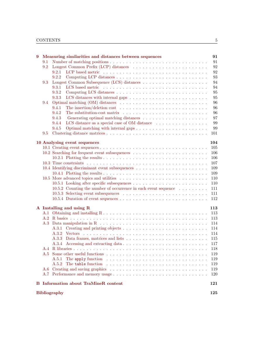
CONTENTS 9 Measuring similarities and distances between sequences 9.1 Number of matching positions . . . . . . . . . . . . . . . . . . . . . . . . . . . . . . 9.2 Longest Common Prefix (LCP) distances . . . . . . . . . . . . . . . . . . . . . . . 9.2.1 LCP based metric . . . . . . . . . . . . . . . . . . . . . . . . . . . . . . . . 9.2.2 Computing LCP distances . . . . . . . . . . . . . . . . . . . . . . . . . . . . 9.3 Longest Common Subsequence (LCS) distances . . . . . . . . . . . . . . . . . . . . 9.3.1 LCS based metric . . . . . . . . . . . . . . . . . . . . . . . . . . . . . . . . 9.3.2 Computing LCS distances . . . . . . . . . . . . . . . . . . . . . . . . . . . . 9.3.3 LCS distances with internal gaps . . . . . . . . . . . . . . . . . . . . . . . . . . . . . . . . . . . . . . . . . . . . . . . . . . . 9.4 Optimal matching (OM) distances 9.4.1 The insertion/deletion cost . . . . . . . . . . . . . . . . . . . . . . . . . . . 9.4.2 The substitution-cost matrix . . . . . . . . . . . . . . . . . . . . . . . . . . 9.4.3 Generating optimal matching distances . . . . . . . . . . . . . . . . . . . . 9.4.4 LCS distance as a special case of OM distance . . . . . . . . . . . . . . . . 9.4.5 Optimal matching with internal gaps . . . . . . . . . . . . . . . . . . . . . . 9.5 Clustering distance matrices . . . . . . . . . . . . . . . . . . . . . . . . . . . . . . . 10 Analysing event sequences 10.1 Creating event sequences . . . . . . . . . . . . . . . . . . . . . . . . . . . . . . . . . 10.2 Searching for frequent event subsequences . . . . . . . . . . . . . . . . . . . . . . . 10.2.1 Plotting the results . . . . . . . . . . . . . . . . . . . . . . . . . . . . . . . . 10.3 Time constraints . . . . . . . . . . . . . . . . . . . . . . . . . . . . . . . . . . . . . 10.4 Identifying discriminant event subsequences . . . . . . . . . . . . . . . . . . . . . . 10.4.1 Plotting the results . . . . . . . . . . . . . . . . . . . . . . . . . . . . . . . . . . . . . . . . . . . . . . . . . . . . . . . . . . . 10.5.1 Looking after specific subsequences . . . . . . . . . . . . . . . . . . . . . . . 10.5.2 Counting the number of occurrence in each event sequence . . . . . . . . . 10.5.3 Selecting event subsequences . . . . . . . . . . . . . . . . . . . . . . . . . . 10.5.4 Duration of event sequences . . . . . . . . . . . . . . . . . . . . . . . . . . . 10.5 More advanced topics and utilities A Installing and using R A.1 Obtaining and installing R . . . . . . . . . . . . . . . . . . . . . . . . . . . . . . . . A.2 R basics . . . . . . . . . . . . . . . . . . . . . . . . . . . . . . . . . . . . . . . . . . A.3 Data manipulation in R . . . . . . . . . . . . . . . . . . . . . . . . . . . . . . . . . A.3.1 Creating and printing objects . . . . . . . . . . . . . . . . . . . . . . . . . . A.3.2 Vectors . . . . . . . . . . . . . . . . . . . . . . . . . . . . . . . . . . . . . . A.3.3 Data frames, matrices and lists . . . . . . . . . . . . . . . . . . . . . . . . . A.3.4 Accessing and extracting data . . . . . . . . . . . . . . . . . . . . . . . . . . A.4 R libraries . . . . . . . . . . . . . . . . . . . . . . . . . . . . . . . . . . . . . . . . . A.5 Some other useful functions . . . . . . . . . . . . . . . . . . . . . . . . . . . . . . . A.5.1 The apply function . . . . . . . . . . . . . . . . . . . . . . . . . . . . . . . A.5.2 The table function . . . . . . . . . . . . . . . . . . . . . . . . . . . . . . . A.6 Creating and saving graphics . . . . . . . . . . . . . . . . . . . . . . . . . . . . . . A.7 Performance and memory usage . . . . . . . . . . . . . . . . . . . . . . . . . . . . . B Information about TraMineR content Bibliography 5 91 91 92 92 93 94 94 95 95 96 96 96 97 99 99 101 104 105 106 106 107 109 109 110 110 111 111 112 113 113 113 114 114 114 115 117 118 119 119 119 119 120 121 125
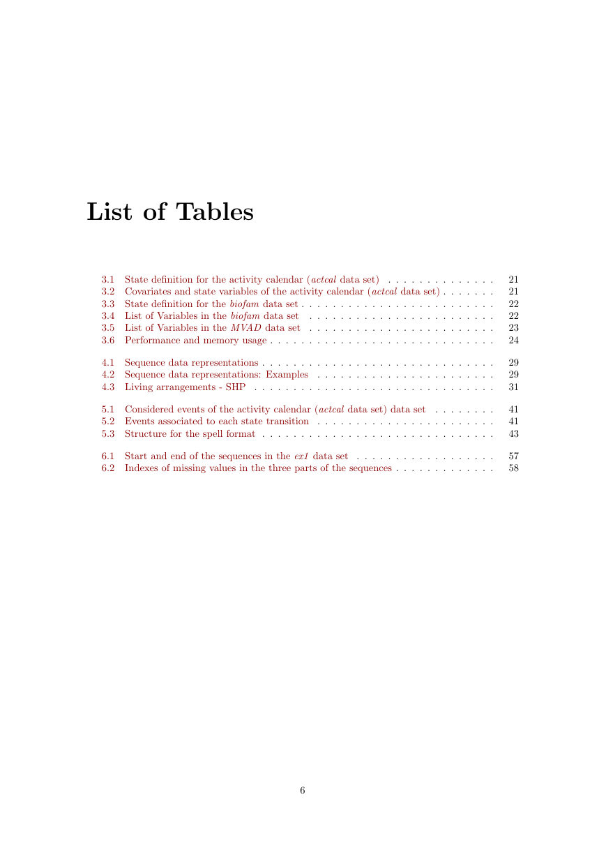
List of Tables 3.1 State definition for the activity calendar (actcal data set) . . . . . . . . . . . . . . 3.2 Covariates and state variables of the activity calendar (actcal data set) . . . . . . . 3.3 State definition for the biofam data set . . . . . . . . . . . . . . . . . . . . . . . . . . . . . . . . . . . . . . . . . . . . . . . . . 3.4 List of Variables in the biofam data set 3.5 List of Variables in the MVAD data set . . . . . . . . . . . . . . . . . . . . . . . . 3.6 Performance and memory usage . . . . . . . . . . . . . . . . . . . . . . . . . . . . . 4.1 Sequence data representations . . . . . . . . . . . . . . . . . . . . . . . . . . . . . . 4.2 Sequence data representations: Examples . . . . . . . . . . . . . . . . . . . . . . . 4.3 Living arrangements - SHP . . . . . . . . . . . . . . . . . . . . . . . . . . . . . . . 5.1 Considered events of the activity calendar (actcal data set) data set . . . . . . . . 5.2 Events associated to each state transition . . . . . . . . . . . . . . . . . . . . . . . 5.3 Structure for the spell format . . . . . . . . . . . . . . . . . . . . . . . . . . . . . . 6.1 Start and end of the sequences in the ex1 data set 6.2 . . . . . . . . . . . . . . . . . . Indexes of missing values in the three parts of the sequences . . . . . . . . . . . . . 21 21 22 22 23 24 29 29 31 41 41 43 57 58 6
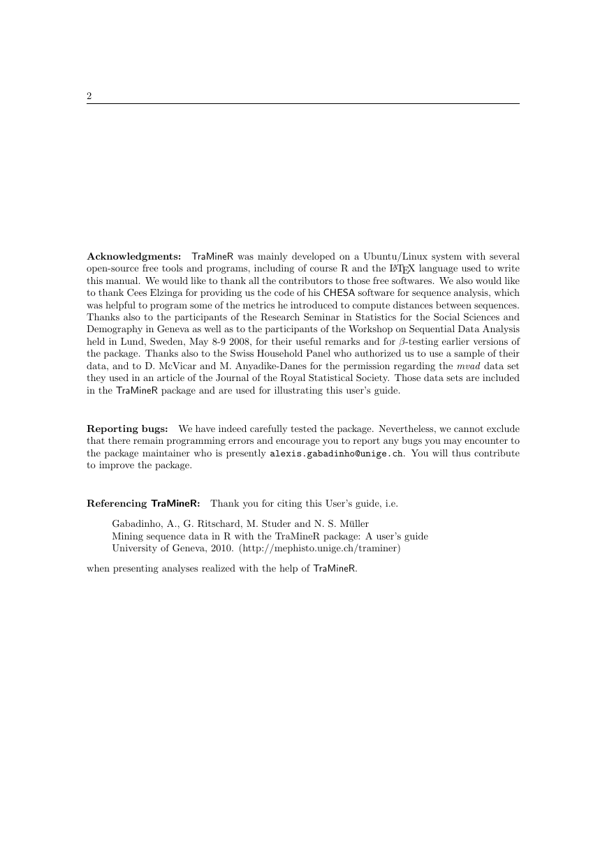
List of Figures sequences (top-right) and state distribution plot (bottom-left) - mvad data set 2.1 A short example - Plot of 10 first sequences (top-left), plot of 10 most frequent . . 2.2 A short example - Entropy of the state distribution (left) and and histogram of sequence turbulence (right) - mvad data set . . . . . . . . . . . . . . . . . . . . . . 2.3 A short example - State distribution within each cluster (mvad data) . . . . . . . . 2.4 A short example - Sequence frequencies whithin each cluster (mvad data) . . . . . 2.5 A short example - Frequencies of most frequent transitions (mvad data) . . . . . . 2.6 A short example - Most discriminating transitions between clusters (mvad data) . 4.1 First 10 sequences of the actcal data (first at bottom) . . . . . . . . . . . . . . . . 4.2 Ontology of types of longitudinal data . . . . . . . . . . . . . . . . . . . . . . . . . 12 13 14 15 16 17 26 28 Swiss Household Panel) 7.1 Legend plotted as an additional graphic . . . . . . . . . . . . . . . . . . . . . . . . 7.2 Distribution of the statuses by age in the mvad data set . . . . . . . . . . . . . . . 7.3 Distribution of the work statuses by month in the actcal data set (data from the . . . . . . . . . . . . . . . . . . . . . . . . . . . . . . . . . 7.4 Entropy of state distribution by age - biofam data set . . . . . . . . . . . . . . . . 7.5 Plot of the 10 most frequent sequences in the actcal data set . . . . . . . . . . . . 7.6 Plot of the 10 most frequent sequences in the biofam data set (bar widths propor- . . . . . . . . . . . . . . . . . . . . . . . . . . . 69 7.7 Mean time spent in each state, actcal data. . . . . . . . . . . . . . . . . . . . . . . 71 7.8 Plot of the 10 first sequences of the actcal data set . . . . . . . . . . . . . . . . . . 72 7.9 Plot of all sequences of the mvad data set, grouped according to the gcse5eq variable 73 tional to the sequence frequencies) 63 65 66 68 68 8.1 Within sequence entropies - actcal data set . . . . . . . . . . . . . . . . . . . . . . 8.2 Within sequence entropies - biofam data set . . . . . . . . . . . . . . . . . . . . . . 8.3 Low, median and high sequence entropies - biofam data set . . . . . . . . . . . . . 8.4 Boxplot of the within sequence entropies by birth cohort - biofam data set . . . . . 8.5 Boxplot of the within sequence entropies by sex - biofam data set . . . . . . . . . . 8.6 Histogram of the sequence turbulences - biofam data set . . . . . . . . . . . . . . . 8.7 Correlation between within sequence turbulence and entropy - biofam data set . . 8.8 Low, median and high sequence turbulences - biofam data set . . . . . . . . . . . . 9.1 Hierarchical sequence clustering from the OM distances, Ward method . . . . . . . 9.2 Sequence frequencies, by cluster - biofam data set . . . . . . . . . . . . . . . . . . . 9.3 Mean time in each state, by cluster - biofam data set . . . . . . . . . . . . . . . . . 10.1 Frequencies of 15 most frequent event subsequences . . . . . . . . . . . . . . . . . . 10.2 Five most discriminating event subsequences between those born before and after 1945. . . . . . . . . . . . . . . . . . . . . . . . . . . . . . . . . . . . . . . . . . . . . 80 81 83 84 84 87 88 90 101 102 103 107 110 7
8 LIST OF FIGURES A.1 R starting welcome message and command prompt . . . . . . . . . . . . . . . . . . 114
分享到:
收藏