Deep learning networks for stock market analysis and prediction_....pdf

发布时间：2022-06-01 发布人：admin 分类：说明书资料大小：2.72M 资料格式：pdf 举报版权申诉

deng0-10367512-4744302543379642607.pdf-第1页.png

第1页 / 共20页

deng0-10367512-4744302543379642607.pdf-第2页.png

第2页 / 共20页

deng0-10367512-4744302543379642607.pdf-第3页.png

第3页 / 共20页

deng0-10367512-4744302543379642607.pdf-第4页.png

第4页 / 共20页

deng0-10367512-4744302543379642607.pdf-第5页.png

第5页 / 共20页

deng0-10367512-4744302543379642607.pdf-第6页.png

第6页 / 共20页

deng0-10367512-4744302543379642607.pdf-第7页.png

第7页 / 共20页

deng0-10367512-4744302543379642607.pdf-第8页.png

第8页 / 共20页

Deep learning networks for stock market analysis and prediction: Methodology, data representations, and case studies

1 Introduction

2 Deep feature learning for stock return prediction

2.1 The framework

2.2 Deep neural network

2.3 Data representation methods

3 Data specification

3.1 Evidence of predictability in the Korean stock market

4 Market representation and trend prediction

4.1 Stock market trend prediction via logistic regression

5 Training deep neural networks

5.1 Performance evaluation

Normalized Mean Squared Error, NMSE

Root Mean Squared Error, RMSE

Mean Absolute Error, MAE

Mutual Information, MI

5.2 Prediction results

5.3 Sensitivity

6 Application to stock market structure analysis

7 Concluding remarks

Acknowledgement

References

Expert Systems With Applications 83 (2017) 187–205 Contents lists available at ScienceDirect Expert Systems With Applications journal homepage: www.elsevier.com/locate/eswa Deep learning networks for stock market analysis and prediction: Methodology, data representations, and case studies Eunsuk Chong ∗ a , a , Chulwoo Han b , Frank C. Park a Robotics Laboratory, Seoul National University, Seoul 08826, Korea b Durham University Business School, Mill Hill Lane, Durham DH1 3LB, UK a r t i c l e i n f o a b s t r a c t Article history: Received 15 November 2016 Revised 15 April 2017 Accepted 16 April 2017 Available online 22 April 2017 Keywords: Stock market prediction Deep learning Multilayer neural network Covariance estimation We offer a systematic analysis of the use of deep learning networks for stock market analysis and pre- diction. Its ability to extract features from a large set of raw data without relying on prior knowledge of predictors makes deep learning potentially attractive for stock market prediction at high frequencies. Deep learning algorithms vary considerably in the choice of network structure, activation function, and other model parameters, and their performance is known to depend heavily on the method of data repre- sentation. Our study attempts to provides a comprehensive and objective assessment of both the advan- tages and drawbacks of deep learning algorithms for stock market analysis and prediction. Using high- frequency intraday stock returns as input data, we examine the effects of three unsupervised feature extraction methods—principal component analysis, autoencoder, and the restricted Boltzmann machine— on the network’s overall ability to predict future market behavior. Empirical results suggest that deep neural networks can extract additional information from the residuals of the autoregressive model and improve prediction performance; the same cannot be said when the autoregressive model is applied to the residuals of the network. Covariance estimation is also noticeably improved when the predictive net- work is applied to covariance-based market structure analysis. Our study offers practical insights and potentially useful directions for further investigation into how deep learning networks can be effectively used for stock market analysis and prediction. © 2017 Elsevier Ltd. All rights reserved. 1. Introduction Research on the predictability of stock markets has a long his- tory in ﬁnancial economics ( e.g., Ang & Bekaert, 2007; Bacchetta, Mertens, & Van Wincoop, 2009; Bondt & Thaler, 1985; Bradley, 1950; Campbell & Hamao, 1992; Campbell & Thompson, 2008; Campbell, 2012; Granger & Morgenstern, 1970 ). While opinions dif- fer on the eﬃciency of markets, many widely accepted empirical studies show that ﬁnancial markets are to some extent predictable ( Bollerslev, Marrone, Xu, & Zhou, 2014; Ferreira & Santa-Clara, 2011; Kim, Shamsuddin, & Lim, 2011; Phan, Sharma, & Narayan, 2015 ). Among methods for stock return prediction, econometric or statistical methods based on the analysis of past market move- ments have been the most widely adopted ( Agrawal, Chourasia, & Mittra, 2013 ). These approaches employ various linear and nonlin- ear methods to predict stock returns, e.g., autoregressive models ∗ Corresponding author. E-mail addresses: bear3498@snu.ac.kr (E. Chong), chulwoo.han@durham.ac.uk (C. Han), fcp@snu.ac.kr (F.C. Park). http://dx.doi.org/10.1016/j.eswa.2017.04.030 0957-4174/© 2017 Elsevier Ltd. All rights reserved. and artiﬁcial neural networks (ANN) ( Adebiyi, Adewumi, & Ayo, 2014; Armano, Marchesi, & Murru, 2005; Atsalakis & Valavanis, 2009; Bogullu, Dagli, & Enke, 2002; Cao, Leggio, & Schniederjans, 2005; Chen, Leung, & Daouk, 2003; Enke & Mehdiyev, 2014; Gure- sen, Kayakutlu, & Daim, 2011a; Kara, Boyacioglu, & Baykan, 2011; Kazem, Shariﬁ, Hussain, Saberi, & Hussain, 2013; Khashei & Bi- jari, 2011; Kim & Enke, 2016a; 2016b; Monfared & Enke, 2014; Rather, Agarwal, & Sastry, 2015; Thawornwong & Enke, 2004; Tic- knor, 2013; Tsai & Hsiao, 2010; Wang, Wang, Zhang, & Guo, 2011; Yeh, Huang, & Lee, 2011; Zhu, Wang, Xu, & Li, 2008 ). While there is uniform agreement that stock returns behave nonlinearly, many empirical studies show that for the most part nonlinear models do not necessarily outperform linear models: e.g., Lee, Sehwan, and Jongdae (2007) , Lee, Chi, Yoo, and Jin (2008) , Agrawal et al. (2013) , and Adebiyi et al. (2014) propose linear models that outperform or perform as well as nonlinear models, whereas Thawornwong and Enke (2004) , Cao et al. (2005) , Enke and Mehdiyev (2013) , and Rather et al. (2015) ﬁnd nonliner models outperfrom linear models. Table 1 provides a summary of recent works relevant to our research. For more exhaustive and detailed reviews, we refer

188 E. Chong et al. / Expert Systems With Applications 83 (2017) 187–205 Table 1 A summery of recent studies on stock market prediction. Authors (Year) Data type (Num. of input features × lagged times) Target output Num. of samples (Training: Validation: Test) Sampling period (Frequency) Method Enke and Mehdiyev (2013) US S&P 500 index (20 × 1) Stock price 361 Jan-1980 to Jan-2010 (daily) Niaki and Hoseinzade (2013) Cervelló-Royo et al. (2015) Korea KOSPI200 × 1) index (27 US Dow Jones × 10) index (1 Market direction (up or down) Market trend (bull/bear-ﬂag) Performance measure RMSE statistical tests Feature + fuzzy selection + clustering fuzzy NN Feature + selection ANN Template matching trading simulation + SVR SVR} {ANN, RF, MAPE, MAE, rRMSE, MSE template Dimension + reduction matching Particle swarm + optimization ANN trading simulation trading simulation Fuzzy system trading simulation {genetic + ANN algorithm, simulated annealing} Deep NN MSE MSE, directional accuracy Dimension + reduction ANN trading simulation, statistical tests Data + representation NN deep NMSE, RMSE, MAE, MI 1-Mar-1994 to 30-Jun-2008 (daily) 22-May-20 0 0 to 29-Nov-2013 (15-min) Jan-2003 to Dec-2012 (daily) 7-Jan-1989 to 24-Mar-2004 (daily) Jan-2008 to Dec-2010 (daily) 15-Nov-1996 to 5-Jun-2012 (daily) Nov-1993 to Jul-2013 (monthly) 2-Sep-2008 to 7-Nov-2008 (1-minute) 1-Jun-2003 to 31-May-2013 (daily) 4-Jan-2010 to 30-Dec-2014 (5-minute) 3650 (8:1:1) 91,307 ∗ 2393 ∗ b , 3412 ∗ a , 3818 (7:0:1) 756 (2:0:1) ∗ 3907 India CNX and BSE indices (10 × 1) Stock price a and × 20) Taiwan TAIEX b US NASDAQ indices (27 World 22 stock market indices ({3 Greece ASE general index (8 × 1) × 1) ∼5} Market trend (bull-ﬂag) Trading signal (stock price) Portfolio composition (cash:stock) Japan Nikkei 225 index (71 × 1) Stock return 237 (7:0:3) × US Apple stock (3 {2 ∼15} + 2) Stock price 19,109 (17:0:3) US SPDR S&P 500 × 1) ETF (SPY) (60 Market direction (up or down) 2518 (14:3:3) Korea KOSPI 38 stock returns (38 × 10) Stock return 73,041 (3:1:1) Patel, Shah, Thakkar, and Kotecha (2015) T.-l. Chen and Chen (2016) Chiang, Enke, Wu, and Wang (2016) Chourmouziadis and Chatzoglou (2016) Qiu, Song, and Akagi (2016) Arévalo, Niño, Hernández, and Sandoval (2016) Zhong and Enke (2017) Our study NN: neural network, SVR: support vector regression, RF: random forest, rRMSE: relative RMSE, NMSE: normalized MSE, MI: mutual information. ∗ In some studies the number of samples is not explicitly provided. We have calculated the number of samples based on each country’s business days. the reader to Atsalakis and Valavanis (2009) , Guresen, Kayakutlu, and Daim (2011b) , and Cavalcante, Brasileiro, Souza, Nobrega, and Oliveira (2016) . Recently there has been a resurgence of interest in artiﬁcial neural networks, in large part to its spectacular successes in image classiﬁcation, natural language processing, and various time-series problems ( Cire ¸s An, Meier, Masci, & Schmidhuber, 2012; Hinton & Salakhutdinov, 2006; Lee, Pham, Largman, & Ng, 2009 ). Underlying this progress is the development of a feature learning framework, known as deep learning ( LeCun, Bengio, & Hinton, 2015 ), whose basic structure is best described as a multi-layer neural network, and whose success can be attributed to a combination of increased computational power, availability of large datasets, and more so- phisticated algorithms ( Bengio, Lamblin, Popovici, Larochelle et al., 2007; Deng & Yu, 2014; Hinton, Osindero, & Teh, 2006; Salakhut- dinov & Hinton, 2009; Srivastava, Hinton, Krizhevsky, Sutskever, & Salakhutdinov, 2014 ). There has been growing interest in whether deep learning can be effectively applied to problems in ﬁnance, but the literature (at 1 With the increas- least in the public domain) still remains limited. ing availability of high-frequency trading data and the less-than- satisfactory performance of existing models, comprehensive studies that objectively examine the suitability of deep learning to stock 1 There exist a few studies that apply deep learning to identiﬁcation of the rela- tionship between past news events and stock market movements ( Ding, Zhang, Liu, & Duan, 2015; Yoshihara, Fujikawa, Seki, & Uehara, 2014 ), but, to our knowledge, there is no study that apply deep learning to extract information from the stock return time series. market prediction and analysis seem opportune. The ability to ex- tract abstract features from data, and to identify hidden nonlinear relationships without relying on econometric assumptions and hu- man expertise, makes deep learning particularly attractive as an alternative to existing models and approaches. ANNs require a careful selection of the input variables and net- work parameters such as the learning rate, number of hidden lay- ers, and number of nodes in each layer in order to achieve satisfac- tory results ( Hussain, Knowles, Lisboa, & El-Deredy, 2008 ). It is also important to reduce dimensionality to improve learning eﬃciency. On the other hand, deep learning automatically extracts features from data and requires minimal human intervention during fea- ture selection. Therefore, our approach does not require expertise on predictors such as macroeconomic variables and enables us to use a large set of raw-level data as input. Ignoring the factors that are known to predict the returns, our approach may not be able to outperform existing models based on carefully chosen predic- tors. However, considering the fast growth of deep learning algo- rithms, we believe our research will serve as a milestone for the future research in this direction. Chourmouziadis and Chatzoglou (2016) also predict that deep learning will play a key role in ﬁnan- cial time series forecasting. We conjecture that, due to correlation, past stock returns affect not only its own future returns but also the future returns of other stocks, and use 380 dimensional lagged stock returns (38 stocks and 10 lagged returns) as input data letting deep learning extract features. This large input dataset makes deep learning a particu- larly suitable choice for our research.

E. Chong et al. / Expert Systems With Applications 83 (2017) 187–205 189 We test our model on high-frequency data from the Korean stock market. Previous studies have predominantly focused on re- turn prediction at a low frequency, and high frequency return prediction studies haven been rare. However, market microstruc- ture noise can cause temporal market ineﬃciency and we ex- pect that many proﬁt opportunities can be found at a high fre- quency. Also, high-frequency trading allows more trading opportu- nities and makes it possible to achieve statistical arbitrage. Another advantage of using high-frequency data is that we can get a large dataset, which is essential to overcome data-snooping and over- ﬁtting problems inevitable in neural network or any other non- linear models. Whilst it should be possible to train the network within 5 min given a reasonable size of training set, we believe daily training should be enough. Put together, the aim of the paper is to assess the potential of deep feature learning as a tool for stock return prediction, and more broadly for ﬁnancial market prediction. Viewed as multi- layer neural networks, deep learning algorithms vary considerably in the choice of network structure, activation function, and other model parameters; their performance is also known to depend heavily on the method of data representation. In this study, we offer a systematic and comprehensive analysis of the use of deep learning. In particular, we use stock returns as input data to a stan- dard deep neural network, and examine the effects of three un- supervised feature extraction methods—principal component anal- ysis, autoencoder, and the restricted Boltzmann machine—on the network’s overall ability to predict future market behavior. The network’s performance is compared against a standard autoregres- sive model and ANN model for high-frequency intraday data taken from the Korean KOSPI stock market. The empirical analysis suggests that the predictive performance of deep learning networks is mixed and depends on a wide range of both environmental and user-determined factors. On the other hand, deep feature learning is found to be particularly effective when used to complement an autoregressive model, considerably improving stock return prediction. Moreover, applying this predic- tion model to covariance-based market structure analysis is also shown to improve covariance estimation effectively. Beyond these ﬁndings, the main contributions of our study are to demonstrate how deep feature learning-based stock return prediction models can be constructed and evaluated, and to shed further light on fu- ture research directions. The remainder of the paper is organized as follows. Section 2 describes the framework for stock return prediction adopted in our research, with a brief review of deep neural net- works and data representation methods. Section 3 describes the sample data construction process using stock returns from the KOSPI stock market. A simple experiment to show evidence of pre- dictability is also demonstrated in this section. Section 4 proposes several data representations that are used as inputs to the deep neural network, and assesses their predictive power via a stock market trend prediction test. Section 5 is devoted to construction and evaluation of the deep neural network; here we compare our model with a standard autoregressive model, and also test a hybrid model that merges the two models. In Section 6 , we apply the results of return predictions to covariance structure analysis, and show that incorporating return predictions improves estimation of correlations between stocks. Concluding remarks with suggestions for the future research are given in Section 7 . 2. Deep feature learning for stock return prediction 2.1. The framework + the stock return at time t For each stock, we seek a predictor function f in order to predict r t+1 , , 1 given the features ( represen- f (u t ) , and the unpredictable part tation ) u t extracted from the information available at time t . We assume that r t+1 can be decomposed into two parts: the predicted = output ˆ r t+1 γ , which we re- gard as Gaussian noise: = + γ ∼ N ˆ r t+1 r t+1 N β ) (0 , where denotes a normal distribution with zero mean and β. The representation u t can be either a linear or a non- variance linear transformation of the raw level information R t . Denoting the transformation function by φ, we have (0 , (1) β ) γ , , φ(R t ) , (2) = u t . ◦ φ(R t ) and = ˆ r t+1 f For our research, we deﬁne the raw level information as the past returns of the stocks in our sample. If there are M stocks in the sample and g lagged returns are chosen, R t will have the form (3) . . . r 1 ,t−g+1 , . . . , , r M,t . . . , r M,t−g+1 ] Mg , R (4) T ∈ = , [ r 1 R t ,t where r i, t denotes the return on stock i at time t . In the remainder of this section, we illustrate the construction of the predictor func- tion f using a deep neural network, and the transformation func- tion φ using different data representation methods. 2.2. Deep neural network , and h l+1 A Neural network speciﬁes the nonlinear relationship between through a network function, which typi- two variables h l cally has the form = + δ(W h l b) h l+1 (5) δ is called an activation function, and the matrix W and where vector b are model parameters. The variables h l are said to form a layer; when there is only one layer between the variables, their relationship is called a single-layer neural network. Multi- layer neural networks augmented with advanced learning methods are generally referred to as deep neural networks (DNN). A DNN = , for the predictor function, y can be constructed by serially stacking the network functions as follows: and h l+1 f (u ) = = h 1 h 2 = y + δ1 ( ) b 1 W 1 u + δ2 ( ) b 2 W 2 h 1 . . . δL ( W L h L where L is the number of layers. , + −1 ) b L { n , u τ n } N =1 n Given a dataset E (y n , f (u n ) of inputs and targets, and an error τ n ) that measures the difference between the out- function n = τ n , the model parameters for the and the target put y θ = , , , , entire network, can be chosen so as to b 1 W L minimize the sum of the errors: { , W 1 } , b L . . . . . . (y n , τ n ) . (6) N E =1 n = J min θ E (·) , its gradient can be obtained Given an appropriate choice of analytically through error backpropagation ( Bishop, 2006 ). In this case, the minimization problem in (6) can be solved by the usual gradient descent method. A typical choice for the objective func- tion that we adopt in this paper has the form: = J N L 2 + λ · (7) y W l l=1 , 2 respectively denote the Euclidean norm and norm. The second term is a “regularizer” added to λ is a user-deﬁned coeﬃcient. 1 N =1 n · n − τ n · and where the matrix L 2 avoid overﬁtting, while 2

190 E. Chong et al. / Expert Systems With Applications 83 (2017) 187–205 2.3. Data representation methods Transforming (representing) raw data before inputing it into a machine learning task often enhances the performance of the task. It is generally accepted that the performance of a machine learn- ing algorithm depends heavily on the choice of the data repre- sentation method ( Bengio, Courville, & Vincent, 2013; Längkvist, Karlsson, & Loutﬁ, 2014 ). There are various data representation methods such as zero-to-one scaling, standardization, log-scaling, and principal component analysis (PCA) ( Atsalakis & Valavanis, 2009 ). More recently, nonlinear methods became popular: Zhong and Enke (2017) compare PCA and two of its nonlinear variants; fuzzy robust PCA and kernel-based PCA. In this paper, we consider three unsupervised data representation methods: PCA, the autoen- coder (AE), and the restricted Boltzmann machine (RBM). PCA in- volves a linear transformation while the other two are nonlinear transformations. These representation methods are widely used in, e.g., image data classiﬁcation ( Coates, Lee, & Ng, 2010 ). For raw data x and a transformation function φ(x ) is called a representation of x , while each element of u is called a → ψ : u x , feature. In some cases we can also deﬁne a reverse map, = ψ (u ) , and retrieve x from u ; in this case the retrieved value, x rec ψ is called a reconstruction of x . The functions can be learned from x and x rec by minimizing the difference (reconstruc- tion error) between them. We now brieﬂy describe each method below. φ and = φ, u R R R (i) Principal Component Analysis, PCA = D via a linear transformation u ∈ ∈ d is generated from the raw In PCA, the representation u ∈ b, data x ∈ d×D , d . The rows of W are and b where W the eigenvectors of the ﬁrst d largest eigenvalues, and b is −W E[ x ] so that E[ u ] = 0 . Reconstruction of usually set to = the original data from the representation is given by x rec − b) ψ (u ) (ii) Autoencoder, AE + W x φ(x ) W W T = T (u W = = I, . R δ = / 1 (W l l (−z) δ . Although + δ(z) (1 AE is a neural network model characterized by a structure in which the model parameters are calibrated by minimiz- + = h l−1 ) be the ing the reconstruction error. Let h l b l network function of the l th layer with input h l−1 and out- can differ across layers, a sigmoid func- put h l l , is typically used for all lay- tion, exp ers, which we also adopt in our research. as a function of the input, the representation of x can be writ- = φ(x ) ten as u x ). Then the reconstruction of the data can be similarly de- = , ﬁned: x rec and the model can be calibrated by minimizing the reconstruction error over a training dataset, . We adopt the following learning criterion: ◦ h 1 (x ) . ◦ h L ◦ . +1 ( h 2 L n } 2 Regarding h l = for an L -layer AE ( h 0 ◦ . h L = { ψ (u ) N =1 n = ) u x ) . . . 2 , || 1 N min θ ◦ φ(x n ) || n − ψ x =1 n } { = θ = , , is often set as the b i where i W i = −i +1 , L, , , i in which case only W i transpose of W L need to be estimated. In this paper, we consider a single- layer AE and estimate both W 1 + , 2 L . W L i and W 2 . (8) , 1 , 1 . . . . . . N (iii) Restricted Boltzmann Machine, RBM RBM ( Hinton, 2002 ) has the same network structure as a single-layer autoencoder, but it uses a different learning method. RBM treats the input and output variables, x and , u , random, and deﬁnes an energy function , from which the joint probability density function of x and u is (x, ) u E determined from the formula (−E (x, Z exp , )) u ) u exp p(x, = = where Z is the partition function. In most cases, u is assumed to be a d -dimensional binary vari- d , and x is assumed to be either binary able, i.e., u or real-valued. When x is a real-valued variable, the energy function has the following form ( Cho, Ilin, & Raiko, 2011 ): ∈ {0, 1} (−E (9) (x, x,u u )) E (x, ) u = − b) T −1 (x − b) (x 1 2 − c T u − u T W −1 / 2 x , (10) , , W, b, c are model parameters. We set = + δ(c j W ( j, + (b i T , u W (: ) ,i i to be where the identity matrix; this makes learning simpler with little performance sacriﬁce ( Taylor, Hinton, & Roweis, 2006 ). From Eqs. (9) and (10) , the conditional distributions are obtained as follows: | = p(u j ) 1 x | = N ) p(x i D, u ·) is the sigmoid function, and W ( j , : ) δ( where are the j th row and the i th column of W , respectively. This type of RBM is denoted the Gaussian–Bernoulli RBM. The input data is then represented and reconstructed in a probabilis- tic way using the conditional distributions. Given an input N =1 , dataset maximum log-likelihood learning is formu- n lated as the following optimization: = , 1 j = , 1 i and W (:, i ) ) x :) 1) (12) (11) d, { x , , , . . . . . . , (13) n } N max θ n ; θ ) = L log p(x c} b, =1 n { W, θ = where are the model parameters, and u is marginalized out ( i.e., integrated out via expectation). This problem can be solved via standard gradient descent. How- ever, due to the computationally intractable partition func- tion Z , an analytic formula for the gradient is usually un- available. The model parameters are instead estimated us- ing a learning method called the contrastive divergence (CD) method ( Carreira-Perpinan & Hinton, 2005 ); we refer the reader to Hinton (2002) for details on learning with RBM. 3. Data speciﬁcation We construct a deep neural network using stock returns from the KOSPI market, the major stock market in South Korea. We ﬁrst choose the ﬁfty largest stocks in terms of market capitaliza- tion at the beginning of the sample period, and keep only the stocks which have a price record over the entire sample period. This leaves 38 stocks in the sample, which are listed in Table 2 . The stock prices are collected every ﬁve minutes during the trad- ing hours of the sample period (04-Jan-2010 to 30-Dec-2014), and ﬁve-minute logarithmic returns are calculated using the formula = t is r t ﬁve minutes. We only consider intraday prediction, i.e., the ﬁrst ten = ﬁve-minute returns ( i.e., lagged returns with g 10 ) each day are used only to construct the raw level input R t , and not included in the target data. The sample contains a total of 1239 trading days and 73,041 ﬁve-minute returns (excluding the ﬁrst ten returns each day) for each stock. , where S t is the stock price at time t , and /S t−t ) (S t ln The training set consists of the ﬁrst 80% of the sample (from ) stock re- 04-Jan-2010 to 24-Dec-2013) which contains 58,421 ( N 1 turns, while the remaining 20% (from 26-Dec-2013 to 30-Dec- 2014) with 14,620 ( N 2 } n i,t+1 r ) returns is used as the test set: = , 1 i } n i,t+1 r Training set: Test set: n , R t n , R t N 1 , =1 n N 2 , =1 n M. { { , . . . 2 exp ( z ) is applied to each element of z . To avoid over-ﬁtting during training, the last 20% of the training set is further separated as a validation set.

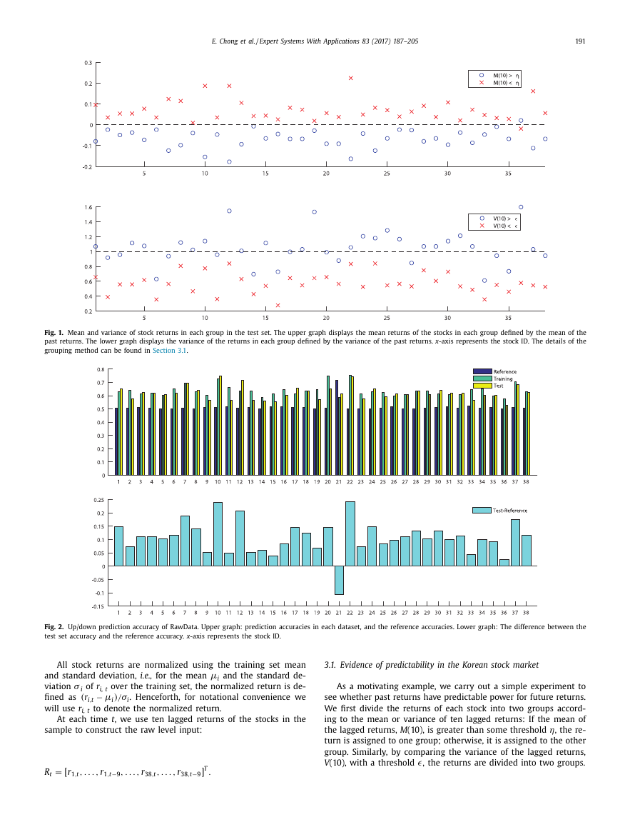
E. Chong et al. / Expert Systems With Applications 83 (2017) 187–205 191 Fig. 1. Mean and variance of stock returns in each group in the test set. The upper graph displays the mean returns of the stocks in each group deﬁned by the mean of the past returns. The lower graph displays the variance of the returns in each group deﬁned by the variance of the past returns. x -axis represents the stock ID. The details of the grouping method can be found in Section 3.1 . Fig. 2. Up/down prediction accuracy of RawData. Upper graph: prediction accuracies in each dataset, and the reference accuracies. Lower graph: The difference between the test set accuracy and the reference accuracy. x -axis represents the stock ID. All stock returns are normalized using the training set mean and the standard de- over the training set, the normalized return is de- ) . Henceforth, for notational convenience we i i and standard deviation, i.e., for the mean σ of r i, t viation − μ i (r i,t ﬁned as to denote the normalized return. will use r i, t /σ μ i At each time t , we use ten lagged returns of the stocks in the sample to construct the raw level input: = , [ r 1 R t ,t . . . , r 1 ,t−9 , . . . , , r 38 ,t . . . , r 38 ,t−9 ] T . 3.1. Evidence of predictability in the Korean stock market As a motivating example, we carry out a simple experiment to see whether past returns have predictable power for future returns. We ﬁrst divide the returns of each stock into two groups accord- ing to the mean or variance of ten lagged returns: If the mean of η, the re- the lagged returns, M (10), is greater than some threshold turn is assigned to one group; otherwise, it is assigned to the other group. Similarly, by comparing the variance of the lagged returns, , the returns are divided into two groups. V (10), with a threshold

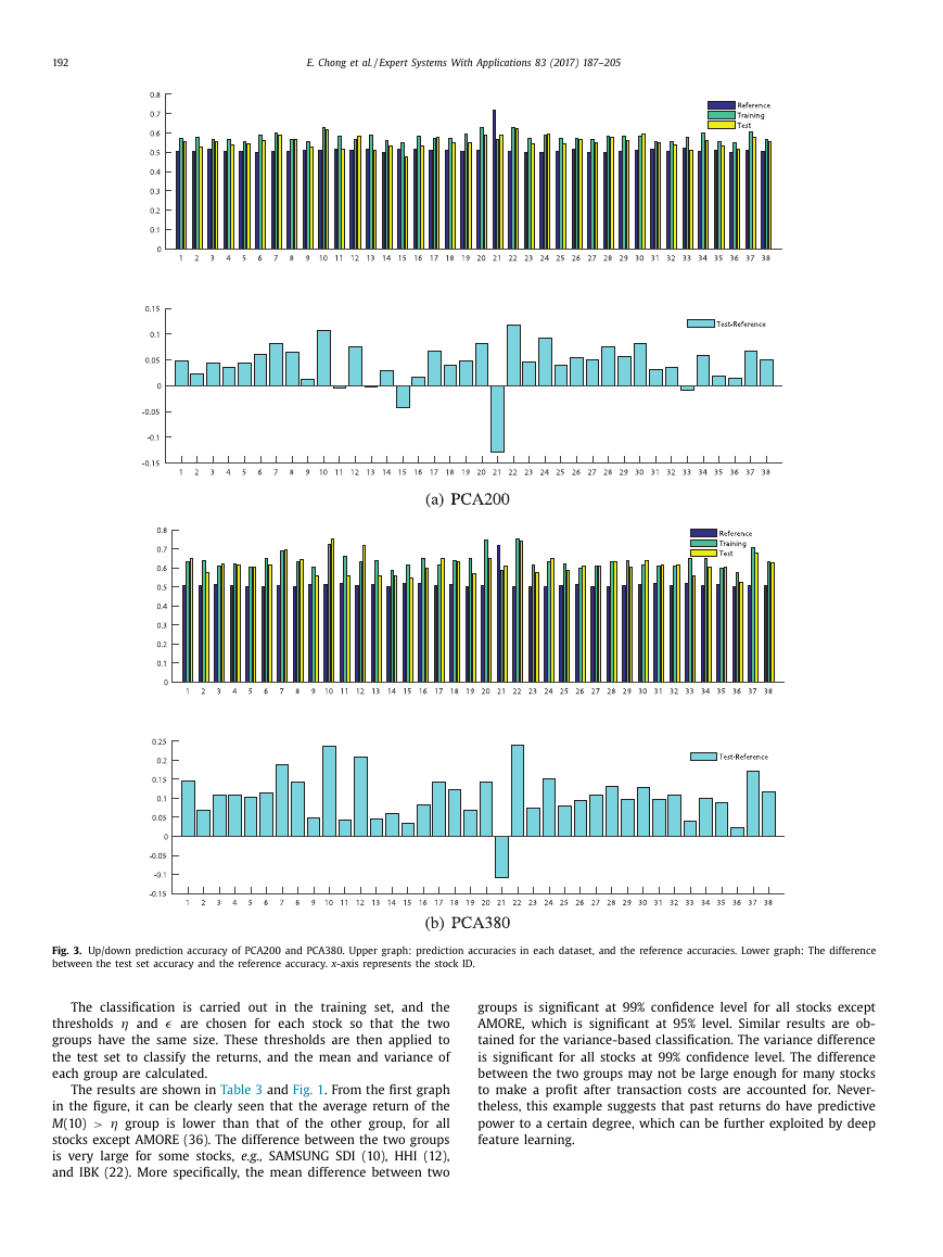
192 E. Chong et al. / Expert Systems With Applications 83 (2017) 187–205 Fig. 3. Up/down prediction accuracy of PCA200 and PCA380. Upper graph: prediction accuracies in each dataset, and the reference accuracies. Lower graph: The difference between the test set accuracy and the reference accuracy. x -axis represents the stock ID. η and The classiﬁcation is carried out in the training set, and the are chosen for each stock so that the two thresholds groups have the same size. These thresholds are then applied to the test set to classify the returns, and the mean and variance of each group are calculated. > The results are shown in Table 3 and Fig. 1 . From the ﬁrst graph in the ﬁgure, it can be clearly seen that the average return of the η group is lower than that of the other group, for all M (10) stocks except AMORE (36). The difference between the two groups is very large for some stocks, e.g., SAMSUNG SDI (10), HHI (12), and IBK (22). More speciﬁcally, the mean difference between two groups is signiﬁcant at 99% conﬁdence level for all stocks except AMORE, which is signiﬁcant at 95% level. Similar results are ob- tained for the variance-based classiﬁcation. The variance difference is signiﬁcant for all stocks at 99% conﬁdence level. The difference between the two groups may not be large enough for many stocks to make a proﬁt after transaction costs are accounted for. Never- theless, this example suggests that past returns do have predictive power to a certain degree, which can be further exploited by deep feature learning.

E. Chong et al. / Expert Systems With Applications 83 (2017) 187–205 193 Fig. 4. Up/down prediction accuracy of RBM400 and RBM800. Upper graph: prediction accuracies in each dataset, and the reference accuracies. Lower graph: The difference between the test set accuracy and the reference accuracy. x -axis represents the stock ID. 4. Market representation and trend prediction In this section, we compare the representation methods de- scribed in Section 2.3 , and analyze their effects on stock return prediction. Each representation method receives the raw level mar- ∈ 380 as the input, and produces the represen- ket movements R t = tation output (features), u t . Several sizes of u t are con- sidered: 200 and 380 for PCA, and 400 and 800 for both RBM and AE. These representations are respectively denoted by PCA200, PCA380, RBM40 0, RBM80 0, AE40 0, and AE80 0 throughout the φ(R t ) R paper. For comparison, the raw level data R t , denote by RawData, is also considered as a representation. Therefore, there are total 7 representations. 4.1. Stock market trend prediction via logistic regression Before training DNN using the features obtained from the rep- resentation methods, we perform a test to assess the predictive power of the features. The test is designed to check whether the features can predict the up/down movement of the future return.

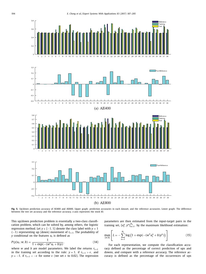
194 E. Chong et al. / Expert Systems With Applications 83 (2017) 187–205 Fig. 5. Up/down prediction accuracy of AE400 and AE800. Upper graph: prediction accuracies in each dataset, and the reference accuracies. Lower graph: The difference between the test set accuracy and the reference accuracy. x -axis represents the stock ID. This up/down prediction problem is essentially a two-class classiﬁ- cation problem, which can be solved by, among others, the logistic ∈ regression method. Let y 1 (−1) representing up (down) movement of r t+1 . The probability of y conditional on the features u t is deﬁned as = denote the class label with y {−1 , 1 } | ; w, (y u t P = b) + exp 1 1 (−(w + b) T u t , ) y (14) where w and b are model parameters. We label the returns r t+1 = in the training set according to the rule: y and = to 0.02). The regression y − for some if r t+1 > , 1 (we set −1 if r t+1 < , , { − N 1 n } = L max { w,b} log =1 n For each representation, we compute the classiﬁcation accu- racy deﬁned as the percentage of correct prediction of ups and downs, and compare with a reference accuracy. The reference ac- curacy is deﬁned as the percentage of the occurrences of ups parameters are then estimated from the input-target pairs in the training set, N 1 =1 , by the maximum likelihood estimation: n n , u y t + exp 1 (−(w n T u t + b) n ) y . (15)

分享到：

赞收藏

资料库

Deep learning networks for stock market analysis and prediction_....pdf

相关推荐

行业

热门标签

最新资料