Notes for ECNU 2007 Short Course
October 2007
0.
Introduction
• Purpose of the course: to offer the students a concise introduction to modern unconstrained and
constrained optimization methods, algorithms, and computer software; functional optimization and
applications will also be briefly addressed.
• Background mathematics includes first-year calculus and linear algebra, some knowledge of calculus of
variations and PDE are helpful but not critical.
• Familiarity with MATLAB is important.
• Most of the distributed course material (Chapters 1, 2, 4, 5, 7, 9, 10, 12, 13, 14, 16, and Appendix A) are
from the book
Andreas Antoniou and Wu-Sheng Lu, Practical Optimization: Algorithms and Engineering Applications,
Springer, New York, March 2007.
The book has a web site: http://www.ece.uvic.ca/~optimization/
I. Numerical Optimization and Applications
1.1 Unconstrained Optimization (Chaps. 1, 2, 4, 5, 7, 9)
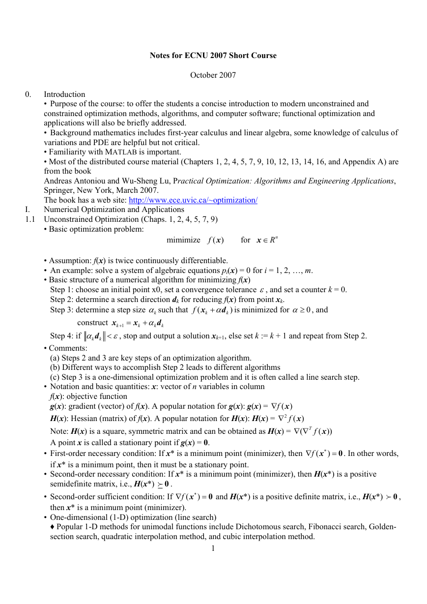
• Basic optimization problem:
x
( )
• Assumption: f(x) is twice continuously differentiable.
• An example: solve a system of algebraic equations pi(x) = 0 for i = 1, 2, …, m.
• Basic structure of a numerical algorithm for minimizing f(x)
mimimize
R∈
for
x
f
n
Step 1: choose an initial point x0, set a convergence tolerance ε, and set a counter k = 0.
Step 2: determine a search direction dk for reducing f(x) from point xk.
d is minimized for
Step 3: determine a step size
k
+
x
+ =
1k
, stop and output a solution xk+1, else set k := k + 1 and repeat from Step 2.
ε
(we illustrate the basic ideas behind the Dichotomous search, Golden-section search, and quadratic
interpolation methods.)
♦ 1-D optimization for general smooth functions: the inexact line search method by Roger Fletcher.
Matlab codes implementing these search methods are available for download at
http://www.ece.uvic.ca/~optimization/
• Determination of a search direction dk:
♦ Basis of the methods: Taylor series of f(x) in a small vicinity surrounding point xk:
f
(
x
k
+
)
δ
=
f
(
x
k
)
T
+ ∇
f
(
x
k
)
or
T
⋅ +
δ δ
2
⋅∇
f
(
x
k
)
⋅ +
δ
O
(
)3
δ
H x
(
)
⋅ +
δ
O
k
(
)3
δ
1
2
1
2
k
k
k
f
(
)
)
(
x
x
+
)
δ
T
⋅ +
δ δ
□ Remarks:
g x
(
T
+
)k
(ii) The steepest descent algorithm is a descent algorithm.
(iii) The steepest descent algorithm is usually quite slow.
f
(
=
⋅
♦ Steepest descent method: dk =
f−∇ x , i.e., dk = –g(xk)
(i) The concept of a descent algorithm
♦ Newton method: dk =
−−H x g x
)
)
+ ≤
1
) (
1(
x
x
(
(
)
f
f
k
k
k
k
H
k
1
I
β
+
β
+
□ Remarks:
(i) if H(xk) = Hk is positive definite for all xk, then the Newton algorithm is a descent algorithm.
(ii) if Hk is not positive definite, then the search direction in Newton method is modified to
with a β such that
H g where ˆ
1ˆ
H
−
k
I
k β+
0
= −
H
=
d
k
k
k
for
k
=
0,1,......
The Newton method with such modifications is a descent algorithm.
(iii) Typically Newton algorithm converges considerably faster than the steepest descent algorithm
at a cost of increased computational intensity.
♦ Quasi-Newton methods: one can take a unifying look at the above two methods as
where
S
k
dk = –Skgk
I
H
1
−
k
for steepest descent
for Newton
⎧
= ⎨
⎩
□ Quasi-Newton methods use gradient information to generate successive low-rank estimation of the
inverse Hessian matrix. In this way, quasi-Newton algorithms provide convergent rates comparable
with that of Newton algorithm with reduced complexity.
□ Notation:
□ Requirements for Sk: (i) Symmetric and positive definite, (ii)
□ Davidon-Fletcher-Powell (DFP) updating formula: S0 = I, and
S γ δ
1k
k
+
δ
k
γ
k
−
=
=
−
=
x
x
g
g
1
+
1
+
,
k
k
k
k
k
S
+ =
1
k
S
k
+
S
S
T
T
δδ
γγ
k
k
k
k
S
T
δ γ γ γ
k
k
k
T
k
−
k
k
k
□ Broyden-Fletcher-Goldfarb-Shanno (BFGS) updating formula: S0 = I, and
S
k
1
+
=
S
k
+
1
+
⎛
⎜
⎝
k
T
T
T
γ γ δδ δγ
k
k
k
γ δ γ δ
k
S
T
k
k
T
k
−
⎞
⎟
⎠
k
k
k
T
γδ
k
k
k
S
S
+
k
T
γ δ
k
k
2
�
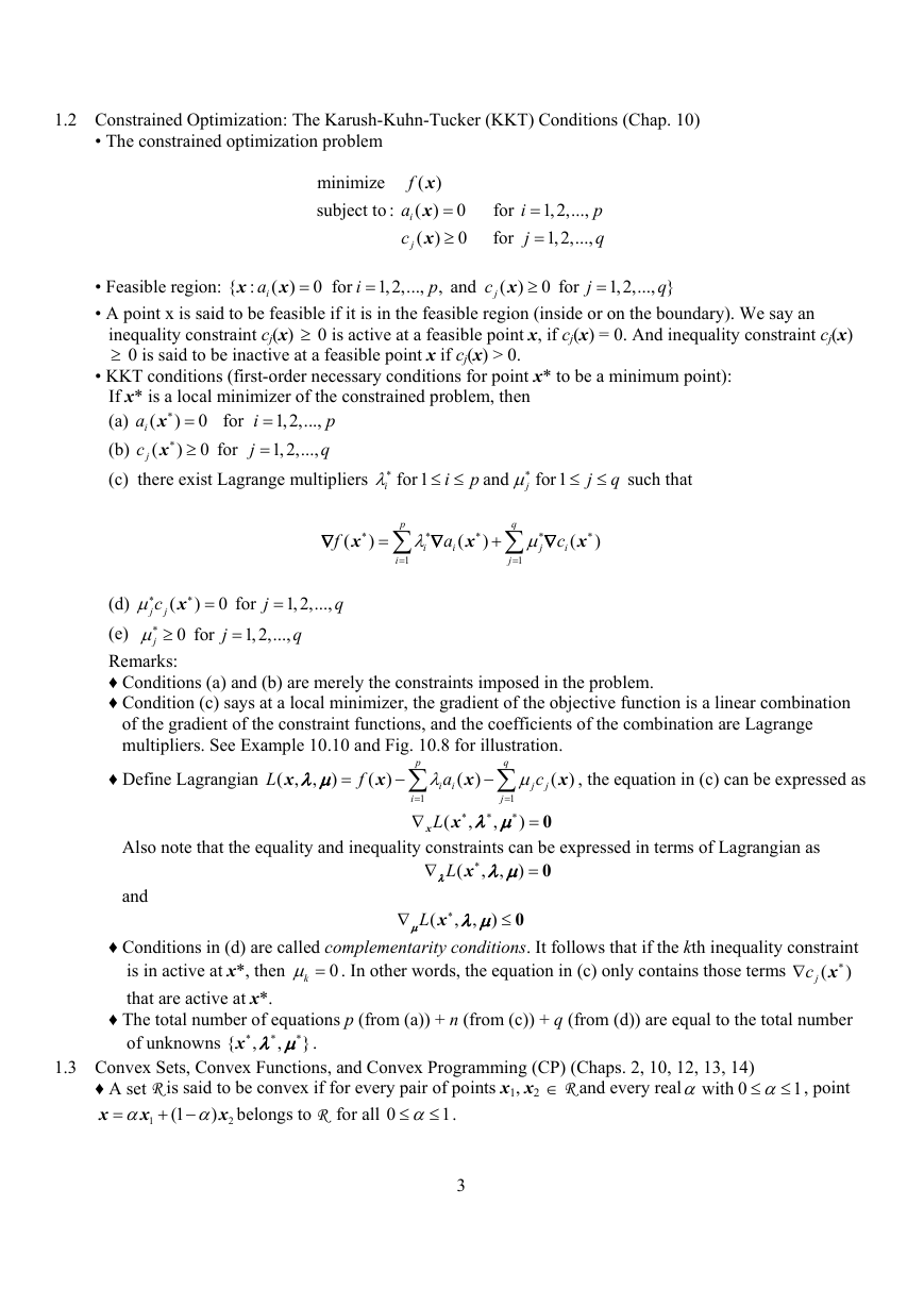
1.2 Constrained Optimization: The Karush-Kuhn-Tucker (KKT) Conditions (Chap. 10)
• The constrained optimization problem
minimize
subject to :
f
a
i
c
j
x
( )
x
( ) 0
=
x
( ) 0
≥
, and
p
for
for
i
j
1,2,...,
=
1,2,...,
=
p
q
j
i
j
c
=
≥
=
=
a
i
1,2,...,
q
1,2,..., }
x
( ) 0 for
x
( ) 0 for
x
• Feasible region: { :
• A point x is said to be feasible if it is in the feasible region (inside or on the boundary). We say an
inequality constraint cj(x) ≥ 0 is active at a feasible point x, if cj(x) = 0. And inequality constraint cj(x)
≥ 0 is said to be inactive at a feasible point x if cj(x) > 0.
• KKT conditions (first-order necessary conditions for point x* to be a minimum point):
If x* is a local minimizer of the constrained problem, then
(a)
(b)
(c) there exist Lagrange multipliers
x
(
) 0 for
∗ =
x
) 0 for
(
∗ ≥
p
1,2,...,
=
q
1,2,...,
=
≤ ≤ such that
for1
for1
ia
jc
≤ ≤
and
∗
μ
j
∗
λ
i
i
j
p
q
i
j
∇
f
∗
(
x
)
=
∗
∇
λ
i
a
i
∗
(
x
)
+
∗
μ
j
∇
c
i
∗
(
x
)
p
∑
i
1
=
q
∑
j
1
=
j
j
q
x
)
∗ =
0 for
0 for
j
=
1,2,...,
1,2,...,
q
jc
(d)
(
μ∗
j
(e)
μ∗ ≥
Remarks:
♦ Conditions (a) and (b) are merely the constraints imposed in the problem.
♦ Condition (c) says at a local minimizer, the gradient of the objective function is a linear combination
of the gradient of the constraint functions, and the coefficients of the combination are Lagrange
=
multipliers. See Example 10.10 and Fig. 10.8 for illustration.
x
♦ Define Lagrangian
( )
)
λμ
x
( )
x
( ,
L
−
=
c
f
,
p
q
μ
j
j
a
λ
i
i
, the equation in (c) can be expressed as
Also note that the equality and inequality constraints can be expressed in terms of Lagrangian as
∑
i
1
=
∇
−
x
( )
∑
1
=
x λ μ
,
∗
,
∗
j
L ∗
(
x
)
= 0
xλ
L ∗
(
∇
,
= 0
λμ
)
,
∇
xμ
L ∗
(
,
≤ 0
λμ
)
,
and
♦ Conditions in (d) are called complementarity conditions. It follows that if the kth inequality constraint
is in active at x*, then
∇ x
jc
)
that are active at x*.
♦ The total number of equations p (from (a)) + n (from (c)) + q (from (d)) are equal to the total number
of unknowns {
kμ = . In other words, the equation in (c) only contains those terms
x λ μ .
}
∗
0
(
,
,
∗
∗
∗
1.3 Convex Sets, Convex Functions, and Convex Programming (CP) (Chaps. 2, 10, 12, 13, 14)
♦ A set R is said to be convex if for every pair of points x1, x2 ∈ R and every real with 0
x
x belongs to R for all 0
2
1α≤
≤ .
(1
+ −
x
α
1
)
α
α
=
α≤ ≤ , point
1
3
�
♦ A function f(x) defined over a convex set R is said to be convex if for every pair of points x1, x2 ∈ R and
every real with 0
≤ ,
α≤
α
1
f
x
(
α
1
(1
+ −
)
α
x
)
≤
f
α
(
x
1
)
2
(1
+ −
)
α
f
(
x
)
2
1C∈ . Function f(x) is convex over a convex set R if and only if
♦ Suppose f(x)
f
(
x
1
)
≥
f
x
( )
+
g
x
( ) (
T
x
1
−
x
)
for all x and x1 ∈ R.
♦ Using the above property, it can be shown that a function f(x)
only if the Hessian H(x) of f(x) is positive semidefinite for x ∈ R.
♦ The problem of minimizing a convex function f(x) (with no constraints) is not very complicated, because
the first-order necessary condition becomes a sufficient condition, and any local minimizer of a convex
function is a global minimizer.
♦ A constrained minimization problem
2C∈ is convex over a convex set R if anf
minimize
subject to :
f
a
i
c
j
x
( )
x
( ) 0
=
x
( ) 0
≥
for
for
i
j
1,2,...,
=
1,2,...,
=
p
q
i
=
=
a
i
1,2,...,
x
( ) 0 for
is said to be a convex programming (CP) problem if the objective function is convex and the feasible
x
q
region defined by the constraints, i.e., { :
1,2,..., }
convex set. In words, a CP problem is a problem of minimizing a convex function over a convex region. It
x
can be shown that the feasible region { :
is
convex if (i) all equality constraint functions ai(x) are linear, and (ii) all inequality functions –cj(x) are
convex.
♦ An important property of the class of CP problems is that the KKT conditions become both necessary
and sufficient. This implies that any {
(minimizer) x* for the CP problem and any local minimizer of a CP problem is a global minimizer.
x λ μ satisfying the KKT conditions gives a local solution
∗
x
( ) 0 for
x
( ) 0 for
x
( ) 0 for
q
1,2,..., }
1,2,...,
, and
, and
is a
a
i
≥
=
=
=
≥
=
p
p
}
c
c
j
i
j
,
,
∗
∗
j
j
1.4 Wolfe Duality (Chap. 10)
Wolfe’s theorem (1991) on duality is concerned with the general CP problem
(P)
which is referred as the primal problem. Wolfe’s theorem says that if {
for the primal problem, then {
x λ μ also solves the dual problem which is defined by
∗
}
∗
∗
− =
b
i
0
for
for
i
j
1,2,...,
=
1,2,...,
=
x λ μ solve the KKT system
∗
p
q
,
,
∗
subject to :
minimize
a
i
c
x
( )
a x
x
( )
T
i
x
( ) 0
f
=
≥
j
,
,
∗
maximize
x
,
λμ
,
}
L
x
( ,
)
λμ
,
(D)
subject to :
)
λμ
,
=
0
x
L∇
( ,
x
0
μ
≥
f
)
(
L
=x
∗
In addition,
♦ Proof: From the KKT conditions of the primal problem, we obtain
For a feasible set { ,
x λμ , we have ≥ 0μ and
x λ μ .
)
∗
, }
(
)
,
,
∗
∗
L
(
x
∗
,
∗
∗
λ μ
,
)
=
f
∗
(
x
)
≥
f
∗
(
x
)
,
f
)
(
=x
∗
x λμ , hence
L∇
( ,
x
p
∑
i
4
= 0
q
∑
a
λ
i
i
μ
j
−
−
x
x
c
1
=
1
=
(
)
(
)
=
∗
∗
j
j
L
(
x λ μ and
∗
)
,
,
∗
∗
∗ ≥ 0μ .
L
(
x
∗
,
λμ
)
,
�
∗
,
L
(
x
x
( ,
)
L
L
(
)
∗ ≥
With ≥ 0μ the Lagrangian
x
∗
L
L x λμ is convex, hence
( ,
,
x
λμ
)
,
,
)
)
)
(
T
λμ
λμ
−
+
≥
x
x λ μ solves the dual problem. ■
Therefore
( ,
,
)
}
λμ , i.e., set {
,
,
∗
∗
∗
x
x
x
f
L
♦ If we define the duality gap ( ,
( )
,
( ,
)
λμ , then the KKT conditions imply that
δ
=
−
λμ
x
,
) 0
,
,
) and (
,
δ ∗
∗
∗
λ μ
λμ
δ
=
q
∑
)
. This is because for a feasible set ( ,
x
) 0 for feasible ( ,
≥
x
( ) 0
≥
, and
λ μ
have
)
λμ
,
)
λμ
,
)
λμ
,
λμ
a
λ
i
i
δ
x
( ,
∑
L
x
( ,
L
x
( ,
L
x
( ,
∑
x
( )
x
( )
x
( )
x
( ,
μ
j
∇
μ
j
c
=
∗
x
=
−
∗
,
=
c
j
+
=
f
,
,
,
,
x
q
j
1
=
j
p
i
1
=
x λμ , we
)
j
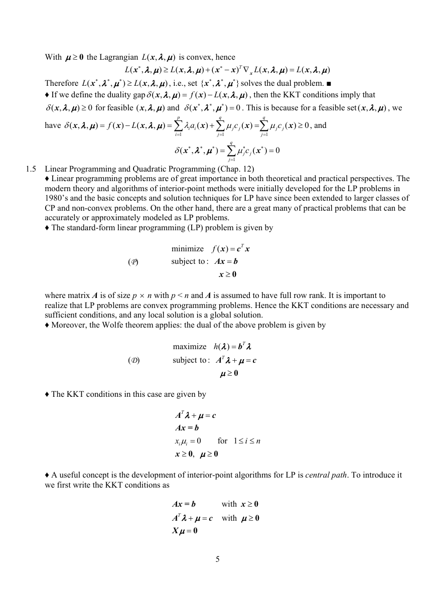
1.5 Linear Programming and Quadratic Programming (Chap. 12)
1
=
j
(
δ
x
∗
,
∗
∗
λ μ
,
)
=
∗
μ
j
c
(
∗
x
) 0
=
j
1
=
q
∑
♦ Linear programming problems are of great importance in both theoretical and practical perspectives. The
modern theory and algorithms of interior-point methods were initially developed for the LP problems in
1980’s and the basic concepts and solution techniques for LP have since been extended to larger classes of
CP and non-convex problems. On the other hand, there are a great many of practical problems that can be
accurately or approximately modeled as LP problems.
♦ The standard-form linear programming (LP) problem is given by
(P)
minimize
subject to :
c x
x
f
( )
T
=
Ax
b
=
x
≥ 0
where matrix A is of size p × n with p < n and A is assumed to have full row rank. It is important to
realize that LP problems are convex programming problems. Hence the KKT conditions are necessary and
sufficient conditions, and any local solution is a global solution.
♦ Moreover, the Wolfe theorem applies: the dual of the above problem is given by
(D)
maximize
subject to :
T
b
h
(
)
λ
=
λ
A
c
T
+ =
λ μ
≥ 0
μ
♦ The KKT conditions in this case are given by
♦ A useful concept is the development of interior-point algorithms for LP is central path. To introduce it
we first write the KKT conditions as
c
+ =
λ μ
A
T
Ax = b
ix
0
μ
=
i
x
0
,
≥
≥
μ
≤ ≤
i
n
for 1
0
x
with
≥
c
with
μ
≥
0
0
Ax = b
A
T
X
λ μ
+ =
0
=
μ
5
�
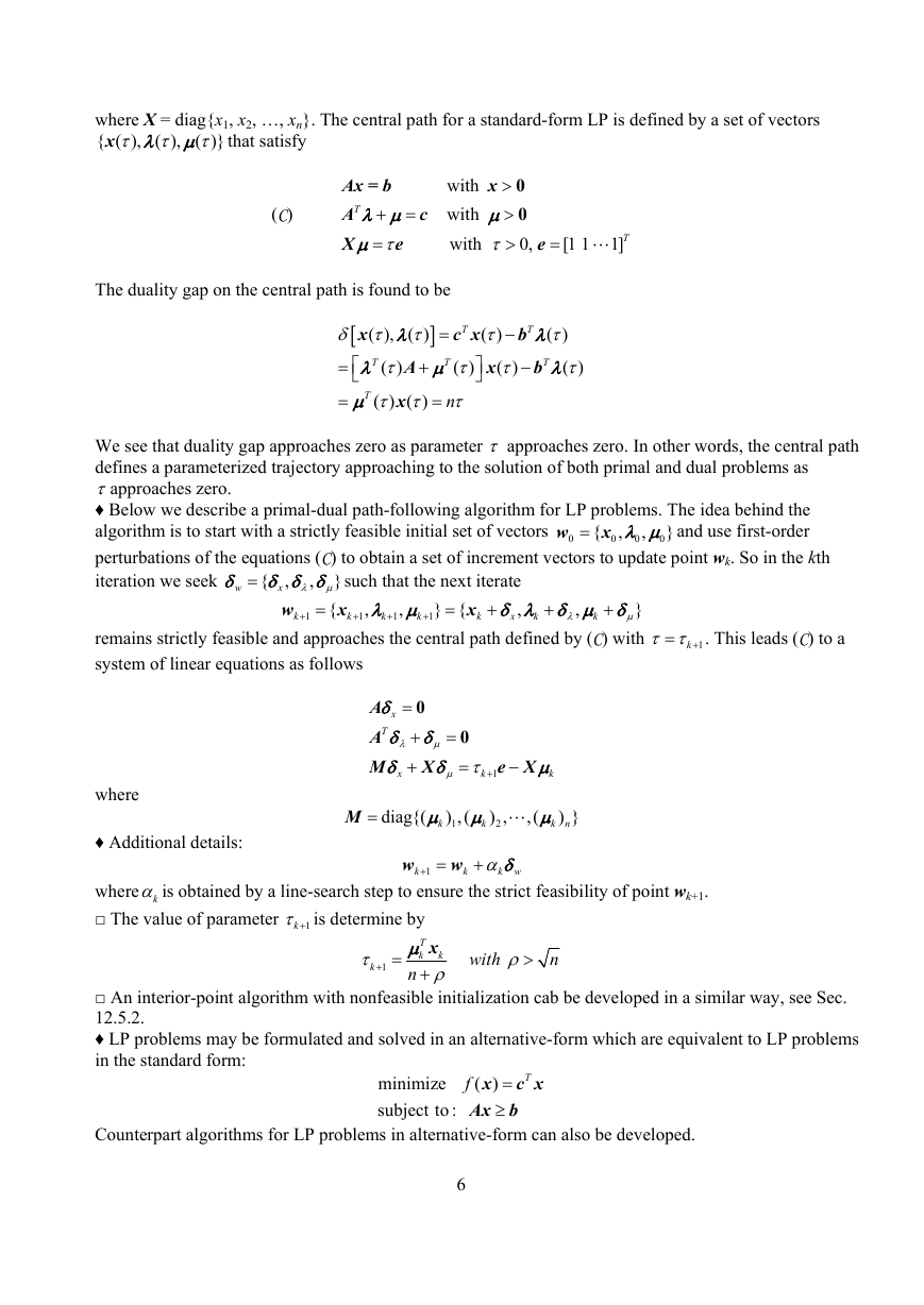
where X = diag{x1, x2, …, xn}. The central path for a standard-form LP is defined by a set of vectors
x λ μ that satisfy
{ ( ),
( )}
τ τ τ
( ),
(C)
Ax = b
A
T
X
+ =
λ μ
e
τ
=
μ
x
with
>
c
with
>
μ
with
τ
>
0
0
0,
e
=
[1 1
1]
T
The duality gap on the central path is found to be
[
]
c x
x
( )
( ),
( )
T
τ
=
δ τ τ
λ
−
x
A
( )
( )
( )
T
T
⎡
⎤
=
μ
λ
+
τ τ
τ
⎦
⎣
x
n
( ) ( )
T
μ
τ τ τ
=
=
b
T
−
( )
λ
τ
b
T
λ
( )
τ
We see that duality gap approaches zero as parameter τ approaches zero. In other words, the central path
defines a parameterized trajectory approaching to the solution of both primal and dual problems as
τapproaches zero.
♦ Below we describe a primal-dual path-following algorithm for LP problems. The idea behind the
x λ μ and use first-order
algorithm is to start with a strictly feasible initial set of vectors
{ ,
0
perturbations of the equations (C) to obtain a set of increment vectors to update point wk. So in the kth
iteration we seek
=w
}
,
0
0
0
,
w
=δ δ δ δ such that the next iterate
,
{ ,
}
x λ μ
x
w
{
=
} {
=
}
δ λ δ μ δ
μ
remains strictly feasible and approaches the central path defined by (C) with
system of linear equations as follows
λ μ
k
,
kλ
+
+
+
x
1
+
1
+
1
+
1
+
,
,
k
k
k
k
x
k
1kτ τ +=
. This leads (C) to a
A
δ
x
A
T
δ δ
=
μ
M
X
e X
−
δ δ
μ τ +
k
1
0
=
+
λ
+
0
=
x
μ
k
where
♦ Additional details:
M
=
diag{(
μ μ
k
) ,(
1
k
) ,
2
,(
μ
) }
k n
w
+ =
1k
w
k
+
δ
k wα
where kα is obtained by a line-search step to ensure the strict feasibility of point wk+1.
□ The value of parameter
1kτ + is determine by
xμ
T
k
k
n
+
ρ
+ =
1
τ
k
with
ρ
>
n
□ An interior-point algorithm with nonfeasible initialization cab be developed in a similar way, see Sec.
12.5.2.
♦ LP problems may be formulated and solved in an alternative-form which are equivalent to LP problems
in the standard form:
minimize
subject to :
c x
x
f
( )
T
=
b
Ax
≥
Counterpart algorithms for LP problems in alternative-form can also be developed.
6
�
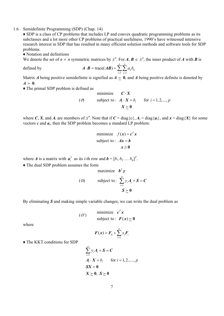
1.6 Semidefinite Programming (SDP) (Chap. 14)
♦ SDP is a class of CP problems that includes LP and convex quadratic programming problems as its
subclasses and a lot more other CP problems of practical usefulness, 1990’s have witnessed intensive
research interest in SDP that has resulted in many efficient solution methods and software tools for SDP
problems.
♦ Notation and definitions
We denote the set of n × n symmetric matrices by S n. For A, B ∈ S n, the inner product of A with B is
defined by
trace(
A B
⋅ =
AB
)
n
n
= ∑∑
a b
ij
ij
i
1
=
j
1
=
Matrix A being positive semidefinite is signified as A 0, and A being positive definite is denoted by
A 0.
♦ The primal SDP problem is defined as
minimize
subject to :
(P)
C X
⋅
A X
⋅
i
X
=
0
ib
for
i
=
1,2,...,
p
where C, X, and Ai are members of S n. Note that if C = diag{c}, Ai = diag{ai}, and x = diag{X} for some
vectors c and ai, then the SDP problem becomes a standard LP problem:
minimize
subject to :
c x
x
f
( )
T
=
b
Ax
=
x
≥ 0
where A is a matrix with
♦ The dual SDP problem assumes the form
T
ia as its i-th row and b = [b1 b2 … bp]T.
maximize
(D)
subject to :
b y
T
p
∑
1
=
S
i
0
y
i
A S C
i
+ =
By eliminating S and making simple variable changes, we can write the dual problem as
(D’)
minimize
subject to :
c x
T
F x
( )
0
where
♦ The KKT conditions for SDP
F x
( )
=
F
0
p
+∑
i
1
=
x
i
F
i
A S C
i
+ =
p
y
i
∑
i
1
=
A X
=
⋅
i
SX
0
=
X
0
,
b
i
for
i
=
1,2.,...,
p
S
0
7
�
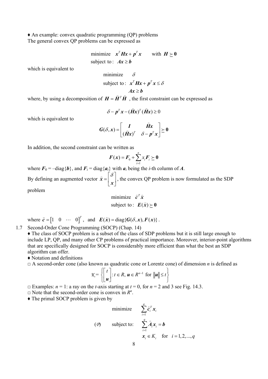
♦ An example: convex quadratic programming (QP) problems
The general convex QP problems can be expressed as
minimize
subject to :
x Hx
T
Ax
≥
p x
T+
b
with
H
0
which is equivalent to
minimize
subject to :
where, by using a decomposition of
H H H , the first constraint can be expressed as
=
T
which is equivalent to
δ−
)T
In addition, the second constraint can be written as
(
G
( ,
δ
x
)
δ
x Hx
T
b
Ax
≥
+
p x
T
≤
δ
) 0
≥
(
−
) (
T
p x Hx Hx
T
Hx
p x
T
−
δ
I
Hx
⎡
= ⎢
⎣
0
⎤
⎥
⎦
F x
( )
=
F
0
x
i
F
i
0
n
+∑
i
1
=
δ⎡ ⎤
= ⎢ ⎥
x
⎣ ⎦
c x
T
E x
( )
0
minimize
subject to :
E x
( ) diag{ ( ,
δ
G
where F0 = –diag{b}, and Fi = diag{ai} with ai being the i-th column of A.
By defining an augmented vector
x
, the convex QP problem is now formulated as the SDP
problem
c
where
x F x .
),
( )}
1.7 Second-Order Cone Programming (SOCP) (Chap. 14)
]
0 , and
[
1 0
=
=
T
♦ The class of SOCP problem is a subset of the class of SDP problems but it is still large enough to
include LP, QP, and many other CP problems of practical importance. Moreover, interior-point algorithms
that are specifically designed for SOCP is considerably more efficient than what the best an SDP
algorithm can offer.
♦ Notation and definitions
□ A second-order cone (also known as quadratic cone or Lorentz cone) of dimension n is defined as
K =
:
t R
∈
,
u
∈
R
n
1
−
for
u
≤
t
t
⎡ ⎤
⎢ ⎥
u
⎣ ⎦
⎧
⎨
⎩
⎫
⎬
⎭
□ Examples: n = 1: a ray on the t-axis starting at t = 0, for n = 2 and 3 see Fig. 14.3.
□ Note that the second-order cone is convex in Rn.
♦ The primal SOCP problem is given by
minimize
q
∑
i
1
=
q
c x
T
i
i
A x
i
i
iK
(P)
subject to:
∑
i
1
=
x
∈
i
=
b
for
i
=
1,2,...,
q
8
�




 2023年江西萍乡中考道德与法治真题及答案.doc
 2012年重庆南川中考生物真题及答案.doc
 2013年江西师范大学地理学综合及文艺理论基础考研真题.doc
 2020年四川甘孜小升初语文真题及答案I卷.doc
 2020年注册岩土工程师专业基础考试真题及答案.doc
 2023-2024学年福建省厦门市九年级上学期数学月考试题及答案.doc
 2021-2022学年辽宁省沈阳市大东区九年级上学期语文期末试题及答案.doc
 2022-2023学年北京东城区初三第一学期物理期末试卷及答案.doc
 2018上半年江西教师资格初中地理学科知识与教学能力真题及答案.doc
 2012年河北国家公务员申论考试真题及答案-省级.doc
 2020-2021学年江苏省扬州市江都区邵樊片九年级上学期数学第一次质量检测试题及答案.doc
 2022下半年黑龙江教师资格证中学综合素质真题及答案.doc