Notes and Solutions for: Pattern Recognition by
Sergios Theodoridis and Konstantinos Koutroumbas.
John L. Weatherwax∗
January 19, 2006
Introduction
Here you’ll find some notes that I wrote up as I worked through this excellent book. I’ve
worked hard to make these notes as good as I can, but I have no illusions that they are perfect.
If you feel that that there is a better way to accomplish or explain an exercise or derivation
presented in these notes; or that one or more of the explanations is unclear, incomplete,
or misleading, please tell me.
If you find an error of any kind – technical, grammatical,
typographical, whatever – please tell me that, too. I’ll gladly add to the acknowledgments
in later printings the name of the first person to bring each problem to my attention.
Acknowledgments
Special thanks to (most recent comments are listed first): Karonny F, Mohammad Heshajin
for helping improve these notes and solutions.
All comments (no matter how small) are much appreciated. In fact, if you find these notes
useful I would appreciate a contribution in the form of a solution to a problem that I did
not work, a mathematical derivation of a statement or comment made in the book that was
unclear, a piece of code that implements one of the algorithms discussed, or a correction to
a typo (spelling, grammar, etc) about these notes. Sort of a “take a penny, leave a penny”
type of approach. Remember: pay it forward.
∗wax@alum.mit.edu
1
�
Classifiers Based on Bayes Decision Theory
Notes on the text
Minimizing the average risk
The symbol rk is the expected risk associated with observing an object from class k. This
risk is divided up into parts that depend on what we then do when an object from class k
with feature vector x is observed. Now we only observe the feature vector x and not the true
class label k. Since we must still perform an action when we observe x let λki represent the
loss associated with the event that the object is truly from class k and we decided that it is
from class i. Define rk as the expected loss when an object of type k is presented to us. Then
rk =
=
M
M
Xi=1
Xi=1
λkiP (we classify this object as a member of class i)
λkiZRi
p(x|ωk)dx ,
which is the books equation 2.14. Thus the total risk r is the expected value of the class
dependent risks rk taking into account how likely each class is or
M
M
M
r =
=
=
rkP (ωk)
Xk=1
λkiZRi
Xk=1
Xi=1
Xi=1 ZRi M
Xk=1
M
p(x|ωk)P (ωk)dx
λkip(x|ωk)P (ωk)! dx .
(1)
The decision rule that leads to the smallest total risk is obtained by selecting Ri to be the
region of feature space in which the integrand above is as small as possible. That is, Ri
should be defined as the values of x such that for that value of i we have
M
Xk=1
λkip(x|ωk)P (ωk) <
M
Xk=1
λkjp(x|ωk)P (ωk) ∀j .
In words the index i, when put in the sum above gives the smallest value when compared to
all other possible choices. For these values of x we should select class ωi as our classification
decision.
2
�
Bayesian classification with normal distributions
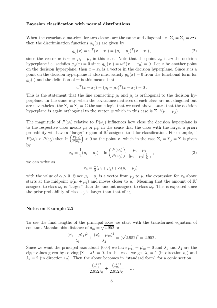
When the covariance matrices for two classes are the same and diagonal i.e. Σi = Σj = σ2I
then the discrimination functions gij(x) are given by
gij(x) = wT (x − x0) = (µi − µj)T (x − x0) ,
(2)
since the vector w is w = µi − µj in this case. Note that the point x0 is on the decision
hyperplane i.e. satisfies gij(x) = 0 since gij(x0) = wT (x0 − x0) = 0. Let x be another point
on the decision hyperplane, then x − x0 is a vector in the decision hyperplane. Since x is a
point on the decision hyperplane it also must satisfy gij(x) = 0 from the functional form for
gij(·) and the definition of w is this means that
wT (x − x0) = (µi − µj)T (x − x0) = 0 .
This is the statement that the line connecting µi and µj is orthogonal to the decision hy-
perplane. In the same way, when the covariance matrices of each class are not diagonal but
are nevertheless the Σi = Σj = Σ the same logic that we used above states that the decision
hyperplane is again orthogonal to the vector w which in this case is Σ−1(µi − µj).
The magnitude of P (ωi) relative to P (ωj) influences how close the decision hyperplane is
to the respective class means µi or µj, in the sense that the class with the larger a priori
probability will have a “larger” region of Rl assigned to it for classification. For example, if
P (ωi) < P (ωj) then ln P (ωi)
P (ωj ) < 0 so the point x0 which in the case Σi = Σj = Σ is given
by
,
(3)
x0 =
we can write as
1
2
P (ωj)
(µi + µj) − ln P (ωi)
µi − µj
||µi − µj||2
Σ−1
x0 =
1
2
(µi + µj) + α(µi − µj) ,
with the value of α > 0. Since µi − µj is a vector from µj to µi the expression for x0 above
starts at the midpoint 1
2(µi + µj) and moves closer to µi. Meaning that the amount of Rl
assigned to class ωj is “larger” than the amount assigned to class ωi. This is expected since
the prior probability of class ωj is larger than that of ωi.
Notes on Example 2.2
To see the final lengths of the principal axes we start with the transformed equation of
constant Mahalanobis distance of dm = √2.952 or
(x′1 − µ′11)2
λ1
+
(x′2 − µ′12)2
λ2
= (√2.952)2 = 2.952 .
Since we want the principal axis about (0, 0) we have µ′11 = µ′12 = 0 and λ1 and λ2 are the
eigenvalues given by solving |Σ − λI| = 0. In this case, we get λ1 = 1 (in direction v1) and
λ2 = 2 (in direction v2). Then the above becomes in “standard form” for a conic section
(x′1)2
2.952λ1
+
(x′2)2
2.952λ2
= 1 .
3
�
From this expression we can read off the lengths of the principle axis
2p2.952λ1 = 2√2.952 = 3.43627
2p2.952λ2 = 2p2.952(2) = 4.85962 .
Maximum A Posteriori (MAP) Estimation: Example 2.4
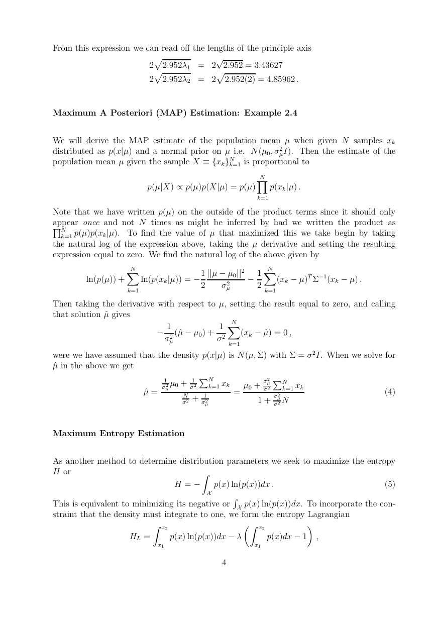
We will derive the MAP estimate of the population mean µ when given N samples xk
distributed as p(x|µ) and a normal prior on µ i.e. N(µ0, σ2
µI). Then the estimate of the
population mean µ given the sample X ≡ {xk}N
k=1 is proportional to
p(µ|X) ∝ p(µ)p(X|µ) = p(µ)
N
Yk=1
p(xk|µ) .
Note that we have written p(µ) on the outside of the product terms since it should only
appear once and not N times as might be inferred by had we written the product as
QN
k=1 p(µ)p(xk|µ). To find the value of µ that maximized this we take begin by taking
the natural log of the expression above, taking the µ derivative and setting the resulting
expression equal to zero. We find the natural log of the above given by
ln(p(µ)) +
N
Xk=1
ln(p(xk|µ)) = −
1
2
||µ − µ0||2
σ2
µ
1
2
−
N
Xk=1
(xk − µ)T Σ−1(xk − µ) .
Then taking the derivative with respect to µ, setting the result equal to zero, and calling
that solution ˆµ gives
1
σ2
µ
−
(ˆµ − µ0) +
1
σ2
N
Xk=1
(xk − ˆµ) = 0 ,
were we have assumed that the density p(x|µ) is N(µ, Σ) with Σ = σ2I. When we solve for
ˆµ in the above we get
1
σ2
µ
ˆµ =
k=1 xk
µ0 + 1
σ2 PN
σ2 + 1
σ2
µ
N
=
Maximum Entropy Estimation
µ0 + σ2
µ
σ2 PN
σ2 N
1 + σ2
µ
k=1 xk
(4)
As another method to determine distribution parameters we seek to maximize the entropy
H or
p(x) ln(p(x))dx .
(5)
H = −ZX
This is equivalent to minimizing its negative or RX
straint that the density must integrate to one, we form the entropy Lagrangian
p(x) ln(p(x))dx. To incorporate the con-
HL =Z x2
x1
p(x) ln(p(x))dx − λZ x2
x1
p(x)dx − 1 ,
4
�
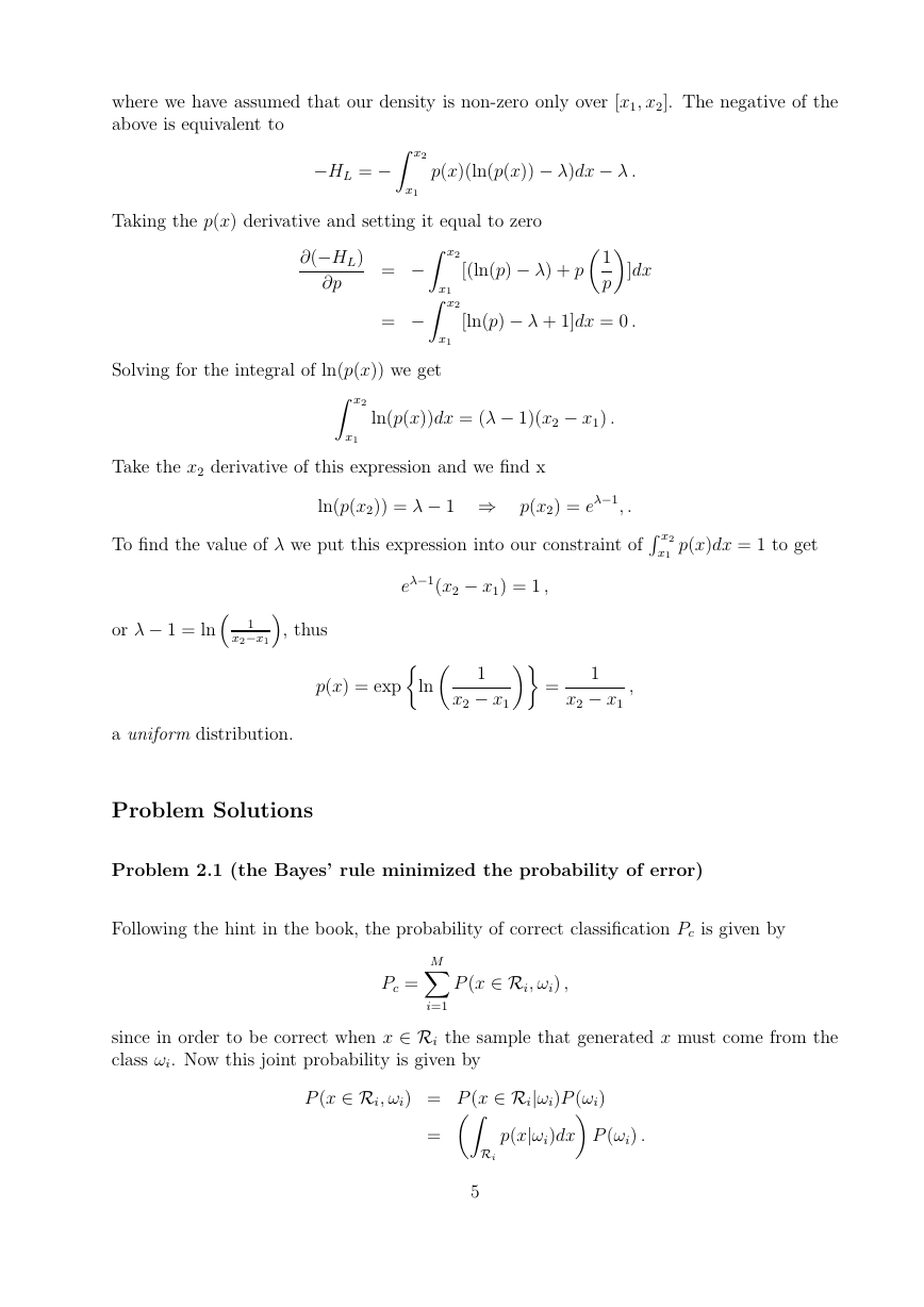
where we have assumed that our density is non-zero only over [x1, x2]. The negative of the
above is equivalent to
−HL = −Z x2
x1
p(x)(ln(p(x)) − λ)dx − λ .
Taking the p(x) derivative and setting it equal to zero
∂(−HL)
∂p
x1
= −Z x2
= −Z x2
x1
p]dx
[(ln(p) − λ) + p1
[ln(p) − λ + 1]dx = 0 .
Solving for the integral of ln(p(x)) we get
Z x2
x1
ln(p(x))dx = (λ − 1)(x2 − x1) .
Take the x2 derivative of this expression and we find x
ln(p(x2)) = λ − 1 ⇒ p(x2) = eλ−1, .
To find the value of λ we put this expression into our constraint of R x2
or λ − 1 = ln 1
x2−x1, thus
eλ−1(x2 − x1) = 1 ,
x1
1
,
p(x) = expln 1
x2 − x1 =
x2 − x1
p(x)dx = 1 to get
a uniform distribution.
Problem Solutions
Problem 2.1 (the Bayes’ rule minimized the probability of error)
Following the hint in the book, the probability of correct classification Pc is given by
Pc =
M
Xi=1
P (x ∈ Ri, ωi) ,
since in order to be correct when x ∈ Ri the sample that generated x must come from the
class ωi. Now this joint probability is given by
P (x ∈ Ri, ωi) = P (x ∈ Ri|ωi)P (ωi)
= ZRi
p(x|ωi)dx P (ωi) .
5
�
So the expression for Pc then becomes
Pc =
=
M
Xi=1 ZRi
Xi=1 ZRi
M
p(x|ωi)dx P (ωi)
p(x|ωi)P (ωi)dx .
(6)
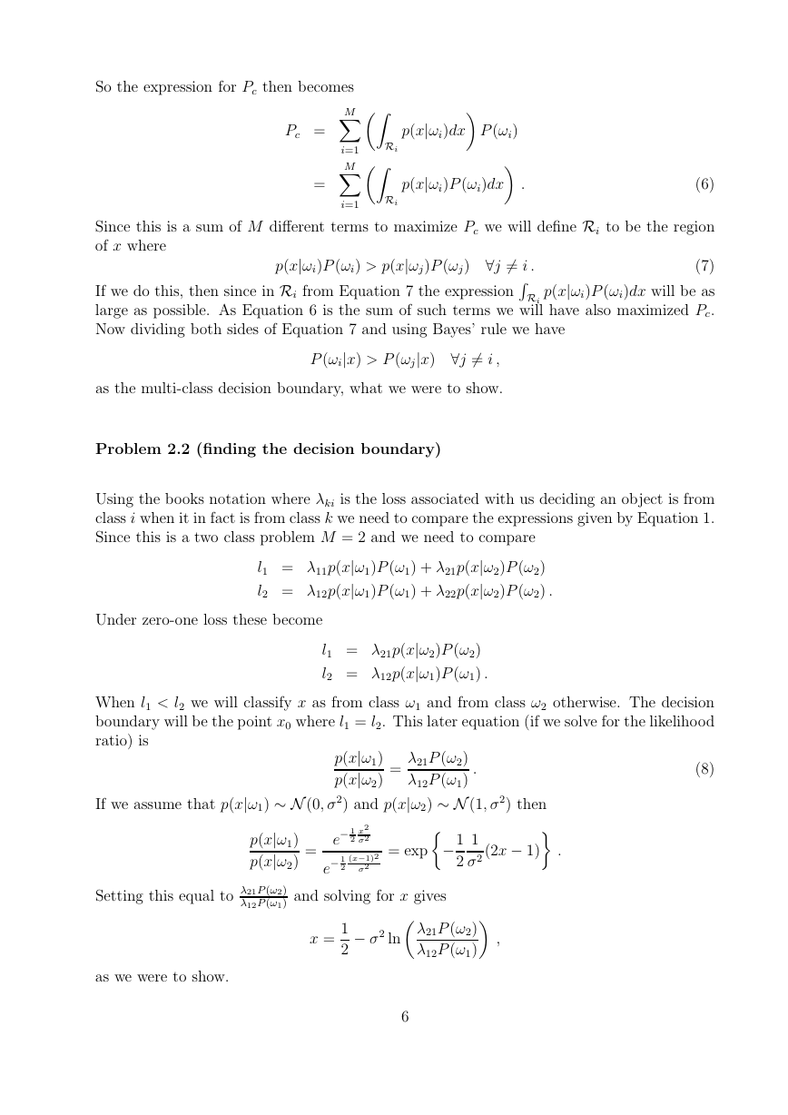
Since this is a sum of M different terms to maximize Pc we will define Ri to be the region
of x where
(7)
p(x|ωi)P (ωi)dx will be as
large as possible. As Equation 6 is the sum of such terms we will have also maximized Pc.
Now dividing both sides of Equation 7 and using Bayes’ rule we have
p(x|ωi)P (ωi) > p(x|ωj)P (ωj) ∀j 6= i .
If we do this, then since in Ri from Equation 7 the expression RRi
P (ωi|x) > P (ωj|x) ∀j 6= i ,
as the multi-class decision boundary, what we were to show.
Problem 2.2 (finding the decision boundary)
Using the books notation where λki is the loss associated with us deciding an object is from
class i when it in fact is from class k we need to compare the expressions given by Equation 1.
Since this is a two class problem M = 2 and we need to compare
l1 = λ11p(x|ω1)P (ω1) + λ21p(x|ω2)P (ω2)
l2 = λ12p(x|ω1)P (ω1) + λ22p(x|ω2)P (ω2) .
Under zero-one loss these become
l1 = λ21p(x|ω2)P (ω2)
l2 = λ12p(x|ω1)P (ω1) .
When l1 < l2 we will classify x as from class ω1 and from class ω2 otherwise. The decision
boundary will be the point x0 where l1 = l2. This later equation (if we solve for the likelihood
ratio) is
=
λ21P (ω2)
λ12P (ω1)
.
(8)
p(x|ω1)
p(x|ω2)
x2
σ2
σ2
If we assume that p(x|ω1) ∼ N (0, σ2) and p(x|ω2) ∼ N (1, σ2) then
σ2 (2x − 1) .
p(x|ω1)
p(x|ω2)
Setting this equal to λ21P (ω2)
λ12P (ω1) and solving for x gives
= exp−
(x−1)2
1
2
2
e− 1
e− 1
2
=
1
as we were to show.
x =
1
λ12P (ω1) ,
2 − σ2 lnλ21P (ω2)
6
�
Problem 2.3 (an expression for the average risk)
We are told to define the errors ε1,2 as the class conditional error or
ε1 = P (x ∈ R2|ω1) =ZR2
ε2 = P (x ∈ R1|ω2) =ZR1
p(x|ω1)dx
p(x|ω2)dx .
Using these definitions we can manipulate the average risk as
p(x|ω1)dx
p(x|ω2)dx
p(x|ω1)dx + λ12ZR2
p(x|ω2)dx + λ22ZR2
r = P (ω1)λ11ZR1
+ P (ω2)λ21ZR1
= P (ω1)λ111 −ZR2
+ P (ω2)λ21ZR1
= λ11P (ω1) − λ11ε1P (ω1) + λ12ε1P (ω1) + λ21ε2P (ω2) + λ22P (ω1) − λ22ε2P (ω2)
= λ11P (ω1) + λ22P (ω2) + (λ12 − λ11)ε1P (ω1) + (λ12 − λ22)ε2P (ω2) ,
p(x|ω1)dx + λ12ZR2
p(x|ω2)dx + λ221 −ZR1
p(x|ω1)dx
p(x|ω2)dx
resulting in the desired expression.
Problem 2.4 (bounding the probability of error)
We desire to show that
Pe ≤ 1 −
1
M
.
To do this recall that since PM
otherwise the sum PM
Bayes’ classification decision. That is
i=1 P (ωi|x) = 1 at least one P (ωi|x) must be larger than 1
i=1 P (ωi|x) would have to be less than one. Now let P (ωi∗|x) be the
M
P (ωi∗|x) = max
i
P (ωi|x) .
From the above discussion P (ωi∗|x) ≥ 1
Pe = 1 − max
i
the desired expression.
M . From this we see that
M − 1
M
P (ωi|x) ≤ 1 −
1
M
=
,
7
�
Problem 2.5 (classification with Gaussians of the same mean)
Since this is a two-class problem we can use the results from the book. We compute l12 the
likelihood ratio
l12 =
(9)
and compare this to the threshold t defined by
p(x|ω1)
p(x|ω2)
=
σ2
2
σ2
1
exp−
x2
2 1
1 −
σ2
1
σ2
2 .
t ≡
P (ω2)
λ12 − λ11 .
P (ω1)λ21 − λ22
Then if l12 > t, then we classify x as a member of ω1. In the same way if l12 < t then we
classify x as a member of ω2. The decision point x0 where we switch classification is given
by l12(x0) = t or
Solving for x0 we get
exp−
x2
0
2 σ2
2 − σ2
1σ2
σ2
2 =
1
σ2
1
σ2
2
t .
x0 = ±
1σ2
2σ2
2
2 − σ2
1)
(σ2
ln σ2
1P (ω2)
σ2
2P (ω1)λ21 − λ22
λ12 − λ11 .
For specific values of the parameters in this problem: σ2
i , P (ωi), and λij the two values for
x0 above can be evaluated. These two values x0 differ only in their sign and have the same
magnitude. For these given values of x0 we see that if |x| ≤ |x0| one class is selected as
the classification decision while if |x| > |x0| the other class is selected. The class selected
depends on the relative magnitude of the parameters σ2
i , P (ωi), and λij and seems difficult
to determine a priori. To determine the class once we are given a fixed specification of these
numbers we can evaluate l12 in Equation 9 for a specific value of x such that |x| ≤ |x0| (say
x = 0) to determine if l12 < t or not. If so the region of x’s given by |x| ≤ |x0| will be
classified as members of class ω1, while the region of x’s where |x| > |x0| would be classified
as members of ω2.
Problem 2.6 (the Neyman-Pearson classification criterion)
Warning:
attempting it. If anyone sees a way to proceed please contact me.
I was not able to solve this problem. Below are a few notes I made while
For this problem we want to fix the value of the error probability for class one at a particular
value say ε1 = ε and then we want to minimize the probability of error we make when
classifying the other class. Now recall the definitions of the error probability εi
and
ε1 =ZR2
ε2 =ZR1
p(x|ω1)P (ω1)dx ,
p(x|ω2)P (ω2)dx .
8
�





 2023年江西萍乡中考道德与法治真题及答案.doc
 2012年重庆南川中考生物真题及答案.doc
 2013年江西师范大学地理学综合及文艺理论基础考研真题.doc
 2020年四川甘孜小升初语文真题及答案I卷.doc
 2020年注册岩土工程师专业基础考试真题及答案.doc
 2023-2024学年福建省厦门市九年级上学期数学月考试题及答案.doc
 2021-2022学年辽宁省沈阳市大东区九年级上学期语文期末试题及答案.doc
 2022-2023学年北京东城区初三第一学期物理期末试卷及答案.doc
 2018上半年江西教师资格初中地理学科知识与教学能力真题及答案.doc
 2012年河北国家公务员申论考试真题及答案-省级.doc
 2020-2021学年江苏省扬州市江都区邵樊片九年级上学期数学第一次质量检测试题及答案.doc
 2022下半年黑龙江教师资格证中学综合素质真题及答案.doc