CHAPTER 12
ROUTING IN SWITCHED NETWORKS
12.1 The average load expected over the course of the busiest hour of use during the
course of a day.
12.2 The tradeoff is between efficiency and resilience.
12.3 A static routing strategy does not adapt to changing conditions on the network but
uses a fixed strategy developed ahead of time. With alternate routing, there are a
number of alternate routes between source and destination and a dynamic choice
of routes is made.
12.4 Correctness, simplicity, robustness, stability, fairness, optimality, and efficiency.
12.5 For fixed routing, a single, permanent route is configured for each source-
destination pair of nodes in the network.
12.6 With flooding, a packet is forwarded to all other switches so that eventually all
routes between source and destination are traversed.
12.7 Advantages: (1) An adaptive routing strategy can improve performance, as seen
by the network user. (2) An adaptive routing strategy can aid in congestion control.
Because an adaptive routing strategy tends to balance loads, it can delay the onset
of severe congestion. Disadvantages: (1) The routing decision is more complex;
therefore, the processing burden on network nodes increases. (2) In most cases,
adaptive strategies depend on status information that is collected at one place but
used at another. There is a tradeoff here between the quality of the information
and the amount of overhead. The more information that is exchanged, and the
more frequently it is exchanged, the better will be the routing decisions that each
node makes. On the other hand, this information is itself a load on the constituent
networks, causing a performance degradation. (3) An adaptive strategy may react
too quickly, causing congestion-producing oscillation, or too slowly, being
irrelevant.
12.8 Given a network of nodes connected by bidirectional links, where each link has a
cost associated with it in each direction, define the cost of a path between two
-56-
�
nodes as the sum of the costs of the links traversed. For each pair of nodes, find a
path with the least cost.
12.9 The Bellman-Ford algorithm uses only on information from its neighbors and
knowledge of its link costs, to update it costs and paths. Dijkstra's algorithm
requires that each node must have complete topological information about the
network; that is, each node must know the link costs of all links in the network.
12.1
The number of hops is one less than the number of nodes visited.
a. The fixed number of hops is 2.
b. The furthest distance from a station is half-way around the loop. On average,
a station will send data half this distance. For an N-node network, the
average number of hops is (N/4) – 1.
1.
c.
12.2 The mean node-node path is twice the mean node-root path. Number the levels of
the tree with the root as 1 and the deepest level as N. The path from the root to
level N requires N – 1 hops and 0.5 of the nodes are at this level. The path from
the root to level N – 1 has 0.25 of the nodes and a length of N – 2 hops. Hence the
mean path length, L, is given by
L =
0.5 (N – 1) + 0.25 (N – 2) + 0.125 (N – 3) + . . .
L =
i1
N 0.5
i
i0.5
i1
i
N 2
Thus the mean node-node path is 2N – 4
12.3 for n := 1 to N do
begin
d[n] := ;
p[n] := -1
end;
d[srce] := 0
insert srce at the head of Q;
{initialization over }
{initialize Q to contain srce only 0}
while Q is not empty do
-57-
�
begin
delete the head node j from Q;
for each link jk that starts at j do
begin
newdist := d[j] + c[j,k];
if newdist < d[k] then
begin
d[k] := newdist;
p[nk] := j
if k Q then insert K at the tail of Q;
end
end;
end;
12.4 This proof is based on one in [BERT92]. Let us claim that
(1) L(i) ≤ L(j) for all i T and j T
(2) For each node j, L(j) is the shortest distance from s to j using paths with all
nodes in T except possibly j.
Condition (1) is satisfied initially, and because w(i, j) ≥ 0 and L(i) = minjT L(j),
it is preserved by the formula in step 3 of the algorithm. Condition (2) then can be
shown by induction. It holds initially. Suppose that condition (2) holds at the
beginning of some iteration. Let i be the node added to T at that iteration, and let
L(k) be the label of each node k at the beginning of the iteration. Condition (2)
holds for i = j by the induction hypothesis, and it holds for all j T by condition (1)
and the induction hypothesis. Finally for a node j T i, consider a path from s to
j which is shortest among all those in which all nodes of the path belong to T i
and let L'(j) be the distance. Let k be the last node of this path before node j. Since k
is in T i, the length of this path from s to k is L(k). So we have
L'(j) = minkTi[w(k, j) +L(k)] = min[minkT[w(k, j) +L(k)], w(i, j) +L(i)]
The induction hypothesis implies that L(j) = minkT[w(k, j) +L(k)], so we have
L'(j) = min[L(j) , w(i, j) +L(i)]
Thus in step 3, L(j) is set to the shortest distance from s to j using paths with all
nodes except j belonging to T i.
12.5 Consider the node i which has path length K+1, with the immediately preceding
node on the path being j. The distance to node i is w(j, i) plus the distance to reach
node j. This latter distance must be L(j), the distance to node j along the optimal
-58-
�
route, because otherwise there would be a route with shorter distance found by
going to j along the optimal route and then directly to i.
12.6 Not possible. A node will not be added to T until its least-cost route is found. As
long as the least-cost route has not been found, the last node on that route will be
eligible for entry into T before the node in question.
12.7 We show the results for starting from node 2.
M
{2}
{2, 4}
{2, 4, 1}
{2, 4, 1, 3}
{2, 4, 1, 3, 5}
{2, 4, 1, 3, 5, 6}
L(1)
3
3
3
3
3
3
Path
2-1
2-1
2-1
2-1
2-1
2-1
L(3)
3
3
3
3
3
3
Path
2-3
2-3
2-3
2-3
2-3
2-3
L(4)
2
2
2
2
2
2
Path
2-4
2-4
2-4
2-4
2-4
2-4
Path
L(5)
L(6)
—
2-4-5
3
3
2-4-5
8
2-4-5
3
5
2-4-5
3
3
2-4-5
5
Path
—
—
—
2-3-6
2-4-5-6
2-4-5-6
1
2
3
4
5
6
-59-
�
12.8 We show the results for starting from node 2.
h
0
1
2
3
4
Lh(1)
3
3
3
3
Path
—
2-1
2-1
2-1
2-1
Lh(3)
3
3
3
3
Path
—
2-3
2-3
2-3
2-3
Lh(4)
2
2
2
2
Path
—
2-4
2-4
2-4
2-4
Lh(5)
3
3
3
Path
—
—
2-4-5
2-4-5
2-4-5
Lh(6)
8
5
5
Path
—
—
2-3-6
2-4-5-6
2-4-5-6
12.9
a. We provide a table for node 1 of network a; the figure is easily generated.
M
{1}
{1,2}
{1,2,5}
{1,2,5,3}
{1,2,5,3,4}
{1,2,5,3,4,6}
L(2) Path L(3)
1
4
1
1
3
3
1
1
3
3
1
1-2
1-2
1-2
1-2
1-2
1-2
Path
—
1-2-3
1-2-5-3
1-2-5-3
1-2-5-3
1-2-5-3
L(4)
4
4
3
3
3
3
Path
1-4
1-4
1-2-5-4
1-2-5-4
1-2-5-4
1-2-5-4
L(5) Path L(6)
—
1-2-5
2
2
1-2-5
6
5
1-2-5
2
2
1-2-5
5
5
1-2-5
2
Path
—
—
1-2-5-6
1-2-5-3-6
1-2-5-3-6
1-2-5-3-6
1
2
3
4
5
6
b. The table for network b is similar in construction but much larger. Here are the
results for node A:
A to B: A-B
A to C: A-B-C
A to D: A-E-G-H-D
A to E: A-E
A to F: A-B-C-F
A to G: A-E-G
A to H: A-E-G-H
A to J: A-B-C-J
A to K: A--E-G-H-D-K
12.10
h
0
1
2
3
4
Lh(2)
1
1
1
1
Path
—
1-2
1-2
1-2
1-2
Lh(3)
4
3
3
Path
—
—
1-2-3
1-2-5-3
1-2-5-3
Lh(4)
4
4
3
3
Path
—
1-4
1-4
1-2-5-4
1-2-5-4
Lh(5) Path Lh(6)
2
2
2
—
—
1-2-5
1-2-5
1-2-5
6
5
Path
—
—
—
1-2-3-6
1-2-5-3-6
12.11 If there is a unique least-cost path, the two algorithms will yield the same result
because they are both guaranteed to find the least-cost path. If there are two or
-60-
�
more equal least-cost paths, the two algorithms may find different least-cost
paths, depending on the order in which alternatives are explored.
12.12 This explanation is taken from [BERT92]. The Floyd-Warshall algorithm iterates
on the set of nodes that are allowed as intermediate nodes on the paths. It starts
like both Dijkstra's algorithm and the Bellman-Ford algorithm with single arc
distances (i.e., no intermediate nodes) as starting estimates of shortest path
lengths. It then calculates shortest paths under the constraint that only node 1
can be used as an intermediate node, and then with the constraint that only
nodes 1 and 2 can be used, and so forth.
For n = 0, the initialization clearly gives the shortest path lengths subject to
the constraint of no intermediate nodes on paths. Now, suppose for a given n,
Ln(i, j) in the above algorithm gives the shortest path lengths using nodes 1 to n
as intermediate nodes. Then the shortest path length from i to j, allowing nodes 1
to n+1 as possible intermediate nodes, either contains node n+1 on the shortest
path or doesn't contain node n+1. For the first case, the constrained shortest path
from i to j goes from i to n+1 and then from n+1 to j, giving the length in the final
term of the equation in step 2 of the problem. For the second case, the
constrained shortest path is the same as the one using nodes 1 to n as possible
intermediate nodes, yielding the length of the first term in the equation in step 2
of the problem.
12.13 a. Consider Figure 12.4, which is valid through part (b). On the third stage, only
5 and 6 are receiving new packets. Node 5 retransmits only to node 6. Thus
the total count is 13 packets.
b. Continue the process beyond Figure 12.4c.
12.14 No. Although it is true that the first packet to reach node 6 has experienced the
minimum delay, this delay was experienced under a condition of network
flooding, and cannot be considered valid for other network conditions.
12.15 The destination node may be unreachable.
12.16 If a node sees a packet arriving on line k from node H with hop count 4, it knows
that H is at most four hops away via line k. If its current best route to H is
estimated at more than four hops, it marks line k as the choice for traffic to H and
records the estimated distance as four hops.
The advantage of this algorithm is that, since it is an isolated technique,
minimal node-node cooperation is needed. The disadvantage occurs if a line
goes down or is overloaded. The algorithm as described only records
improvements, not changes for the worse.
-61-
�
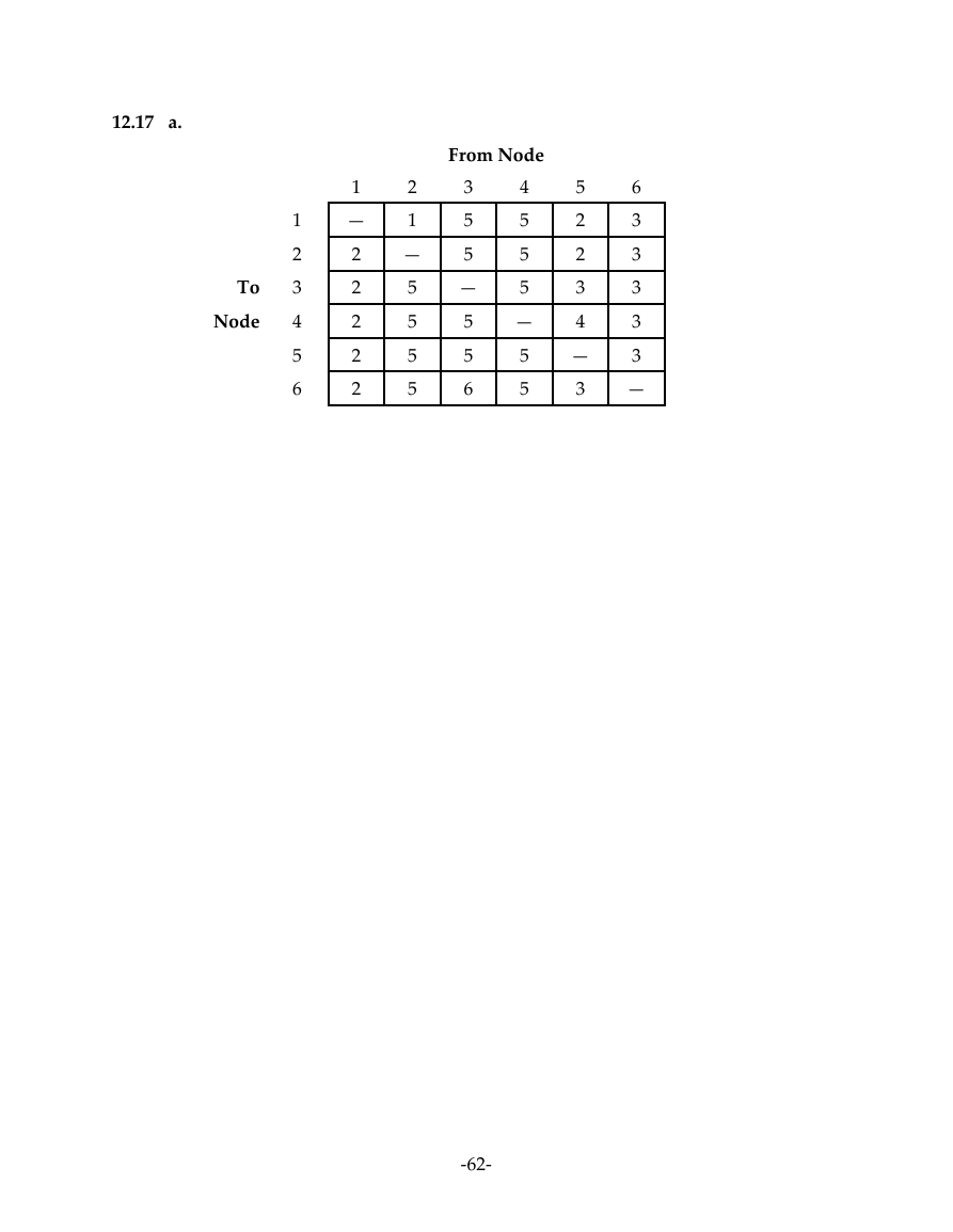
12.17 a.
From Node
1
—
2
2
2
2
2
2
1
—
5
5
5
5
3
5
5
—
5
5
6
4
5
5
5
—
5
5
5
2
2
3
4
—
3
6
3
3
3
3
3
—
1
2
3
4
5
6
To
Node
-62-
�
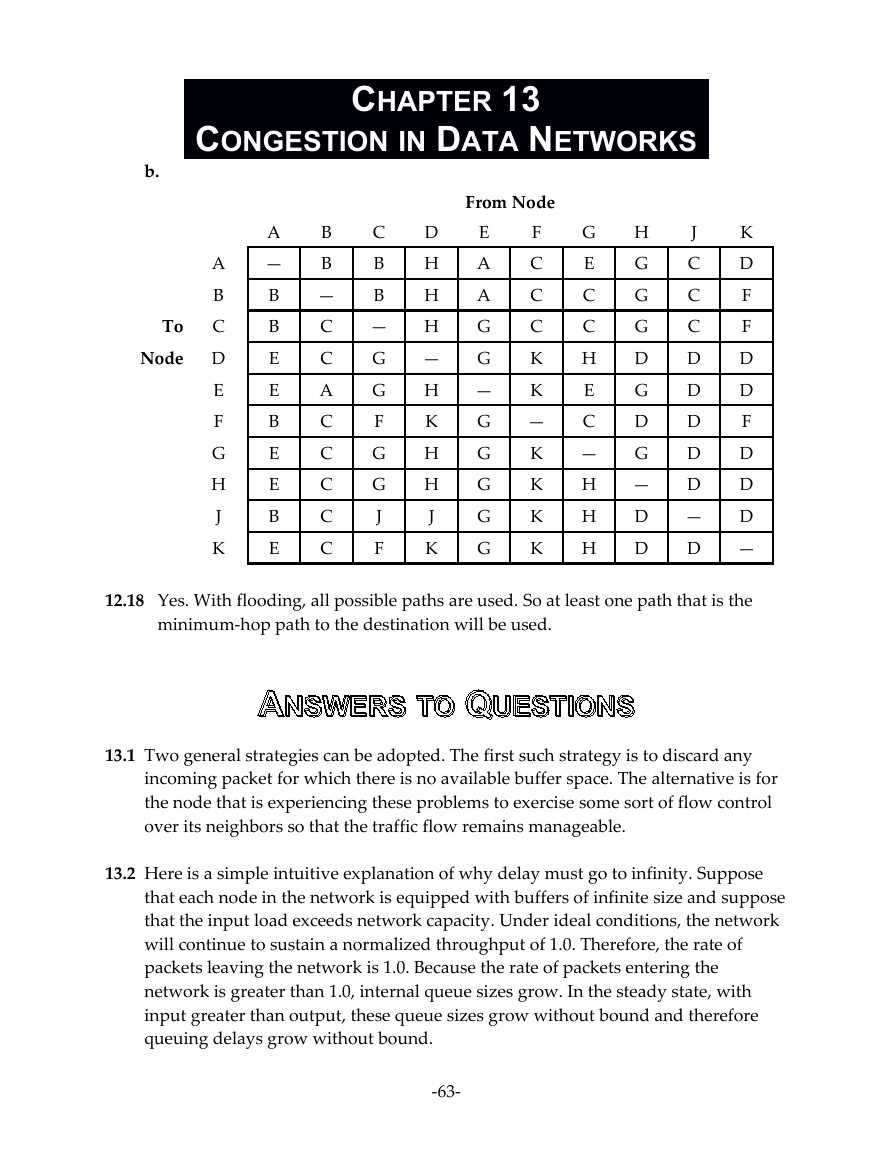
b.
To
Node
CHAPTER 13
CONGESTION IN DATA NETWORKS
A
—
B
B
E
E
B
E
E
B
E
B
B
—
C
C
A
C
C
C
C
C
C
B
B
—
G
G
F
G
G
J
F
A
B
C
D
E
F
G
H
J
K
From Node
D
H
H
H
—
H
K
H
H
J
K
E
A
A
G
G
—
G
G
G
G
G
F
C
C
C
K
K
—
K
K
K
K
G
E
C
C
H
E
C
—
H
H
H
H
G
G
G
D
G
D
G
—
D
D
J
C
C
C
D
D
D
D
D
—
D
K
D
F
F
D
D
F
D
D
D
—
12.18 Yes. With flooding, all possible paths are used. So at least one path that is the
minimum-hop path to the destination will be used.
13.1 Two general strategies can be adopted. The first such strategy is to discard any
incoming packet for which there is no available buffer space. The alternative is for
the node that is experiencing these problems to exercise some sort of flow control
over its neighbors so that the traffic flow remains manageable.
13.2 Here is a simple intuitive explanation of why delay must go to infinity. Suppose
that each node in the network is equipped with buffers of infinite size and suppose
that the input load exceeds network capacity. Under ideal conditions, the network
will continue to sustain a normalized throughput of 1.0. Therefore, the rate of
packets leaving the network is 1.0. Because the rate of packets entering the
network is greater than 1.0, internal queue sizes grow. In the steady state, with
input greater than output, these queue sizes grow without bound and therefore
queuing delays grow without bound.
-63-
�



 2023年江西萍乡中考道德与法治真题及答案.doc
 2012年重庆南川中考生物真题及答案.doc
 2013年江西师范大学地理学综合及文艺理论基础考研真题.doc
 2020年四川甘孜小升初语文真题及答案I卷.doc
 2020年注册岩土工程师专业基础考试真题及答案.doc
 2023-2024学年福建省厦门市九年级上学期数学月考试题及答案.doc
 2021-2022学年辽宁省沈阳市大东区九年级上学期语文期末试题及答案.doc
 2022-2023学年北京东城区初三第一学期物理期末试卷及答案.doc
 2018上半年江西教师资格初中地理学科知识与教学能力真题及答案.doc
 2012年河北国家公务员申论考试真题及答案-省级.doc
 2020-2021学年江苏省扬州市江都区邵樊片九年级上学期数学第一次质量检测试题及答案.doc
 2022下半年黑龙江教师资格证中学综合素质真题及答案.doc