0
2
0
2
r
p
A
1
1
]
G
L
.
s
c
[
1
v
9
3
4
5
0
.
4
0
0
2
:
v
i
X
r
a
1
Meta-Learning in Neural Networks: A Survey
Timothy Hospedales, Antreas Antoniou, Paul Micaelli, Amos Storkey
Abstract—The field of meta-learning, or learning-to-learn, has seen a dramatic rise in interest in recent years. Contrary to
conventional approaches to AI where a given task is solved from scratch using a fixed learning algorithm, meta-learning aims to
improve the learning algorithm itself, given the experience of multiple learning episodes. This paradigm provides an opportunity to
tackle many of the conventional challenges of deep learning, including data and computation bottlenecks, as well as the fundamental
issue of generalization. In this survey we describe the contemporary meta-learning landscape. We first discuss definitions of
meta-learning and position it with respect to related fields, such as transfer learning, multi-task learning, and hyperparameter
optimization. We then propose a new taxonomy that provides a more comprehensive breakdown of the space of meta-learning
methods today. We survey promising applications and successes of meta-learning including few-shot learning, reinforcement learning
and architecture search. Finally, we discuss outstanding challenges and promising areas for future research.
Index Terms—Meta-Learning, Learning-to-Learn, Few-Shot Learning, Transfer Learning, Neural Architecture Search
!
1 INTRODUCTION
Contemporary machine learning models are typically
trained from scratch for a specific task using a fixed learn-
ing algorithm designed by hand. Deep learning-based ap-
proaches have seen great successes in a variety of fields
[1]–[3]. However there are clear limitations [4]. For example,
successes have largely been in areas where vast quantities of
data can be collected or simulated, and where huge compute
resources are available. This excludes many applications
where data is intrinsically rare or expensive [5], or compute
resources are unavailable [6], [7].
Meta-learning provides an alternative paradigm where
a machine learning model gains experience over multiple
learning episodes – often covering a distribution of related
tasks – and uses this experience to improve its future learn-
ing performance. This ‘learning-to-learn’ [8] can lead to a va-
riety of benefits such as data and compute efficiency, and it
is better aligned with human and animal learning [9], where
learning strategies improve both on a lifetime and evo-
lutionary timescale [9]–[11]. Machine learning historically
built models upon hand-engineered features, and feature
choice was often the determining factor in ultimate model
performance [12]–[14]. Deep learning realised the promise
of joint feature and model learning [15], [16], providing a
huge improvement in performance for many tasks [1], [3].
Meta-learning in neural networks can be seen as aiming to
provide the next step of integrating joint feature, model,
and algorithm learning. Neural network meta-learning has a
long history [8], [17], [18]. However, its potential as a driver
to advance the frontier of the contemporary deep learning
industry has led to an explosion of recent research. In
particular meta-learning has the potential to alleviate many
of the main criticisms of contemporary deep learning [4], for
instance by providing better data efficiency, exploitation of
prior knowledge transfer, and enabling unsupervised and
self-directed learning. Successful applications have been
T. Hospedales is with Samsung AI Centre, Cambridge and University of Edin-
burgh. A. Antoniou, P. Micaelli and Storkey are with University of Edinburgh.
Email: {t.hospedales,a.antoniou,paul.micaelli,a.storkey}@ed.ac.uk.
demonstrated in areas spanning few-shot image recognition
[19], [20], unsupervised learning [21], data efficient [22], [23]
and self-directed [24] reinforcement learning (RL), hyper-
parameter optimization [25], and neural architecture search
(NAS) [26]–[28].
Many different perspectives on meta-learning can be
found in the literature. Especially as different communities
use the term somewhat differently, it can be difficult to de-
fine. A perspective related to ours [29] views meta-learning
as a tool to manage the ‘no free lunch’ theorem [30] and
improve generalization by searching for the algorithm (in-
ductive bias) that is best suited to a given problem, or family
of problems. However, taken broadly, this definition can
include transfer, multi-task, feature-selection, and model-
ensemble learning, which are not typically considered as
meta-learning today. Another perspective on meta-learning
[31] broadly covers algorithm selection and configuration
techniques based on dataset features, and becomes hard
to distinguish from automated machine learning (AutoML)
[32]. In this paper, we focus on contemporary neural-network
meta-learning. We take this to mean algorithm or inductive
bias search as per [29], but focus on where this is achieved
by end-to-end learning of an explicitly defined objective function
(such as cross-entropy loss, accuracy or speed).
This paper thus provides a unique, timely, and up-to-
date survey of the rapidly growing area of neural network
meta-learning. In contrast, previous surveys are rather out
of date in this fast moving field, and/or focus on algorithm
selection for data mining [29], [31], [33]–[37], AutoML [32],
or particular applications of meta-learning such as few-shot
learning [38] or neural architecture search [39].
We address both meta-learning methods and applica-
tions. In particular, we first provide a high-level prob-
lem formalization which can be used to understand and
position recent work. We then provide a new taxonomy
of methodologies, in terms of meta-representation, meta-
objective and meta-optimizer. We survey several of the
popular and emerging application areas including few-
shot, reinforcement learning, and architecture search; and
position meta-learning with respect to related topics such
�
as transfer learning, multi-task learning and AutoML. We
conclude by discussing outstanding challenges and areas
for future research.
2 BACKGROUND
Meta-learning is difficult to define, having been used in
various inconsistent ways, even within the contemporary
neural-network literature. In this section, we introduce our
definition and key terminology, which aims to be useful
for understanding a large body of literature. We then po-
sition meta-learning with respect to related topics such as
transfer and multi-task learning, hierarchical models, hyper-
parameter optimization, lifelong/continual learning, and
AutoML.
Meta-learning is most commonly understood as learning
to learn, which refers to the process of improving a learn-
ing algorithm over multiple learning episodes. In contrast,
conventional ML considers the process of improving model
predictions over multiple data instances. During base learn-
ing, an inner (or lower, base) learning algorithm solves a
task such as image classification [15], defined by a dataset
and objective. During meta-learning, an outer (or upper,
meta) algorithm updates the inner learning algorithm, such
that the model learned by the inner algorithm improves
an outer objective. For instance this objective could be
generalization performance or learning speed of the inner
algorithm. Learning episodes of the base task, namely (base
algorithm, trained model, performance) tuples, can be seen
as providing the instances needed by the outer algorithm in
order to learn the base learning algorithm.
As defined above, many conventional machine learning
practices such as random hyper-parameter search by cross-
validation could fall within the definition of meta-learning.
The salient characteristic of contemporary neural-network
meta-learning is an explicitly defined meta-level objective,
and end-to-end optimization of the inner algorithm with
respect to this objective. Often, meta-learning is conducted
on learning episodes sampled from a task family, leading
to a base learning algorithm that is tuned to perform well
on new tasks sampled from this family. This can be a
particularly powerful technique to improve data efficiency
when learning new tasks. However, in a limiting case all
training episodes can be sampled from a single task. In the
following section, we introduce these notions more formally.
2.1 Formalizing Meta-Learning
Conventional Machine Learning
In conventional super-
vised machine learning, we are given a training dataset
D = {(x1, y1), . . . , (xN , yN )}, such as (input image, output
label) pairs. We can train a predictive model ˆy = fθ(x)
parameterized by θ, by solving:
θ∗ = arg min
(1)
where L is a loss function that measures the match between
true labels and those predicted by fθ(·). We include condi-
tion ω to make explicit the dependence of this solution on
factors such as choice of optimizer for θ or function class for
f, which we denote by ω. Generalization is then measured
by evaluating a number of test points with known labels.
L(D; θ, ω)
θ
2
The conventional assumption is that this optimization
is performed from scratch for every problem D; and fur-
thermore that ω is pre-specified. However, the specification
ω of ‘how to learn’ θ can dramatically affect generalization,
data-efficiency, computation cost, and so on. Meta-learning
addresses improving performance by learning the learning
algorithm itself, rather than assuming it is pre-specified and
fixed. This is often (but not always) achieved by revisiting
the first assumption above, and learning from a distribution
of tasks rather than from scratch.
Meta-Learning: Task-Distribution View Meta-learning
aims to improve performance by learning ‘how to learn’ [8].
In particular, the vision is often to learn a general purpose
learning algorithm, that can generalize across tasks and
ideally enable each new task to be learned better than the
last. As such ω specifies ‘how to learn’ and is often evaluated
in terms of performance over a distribution of tasks p(T ).
Here we loosely define a task to be a dataset and loss
function T = {D,L}. Learning how to learn thus becomes
E
L(D; ω)
min
ω
T ∼p(T )
(2)
where L(D; ω) measures the performance of a model
trained using ω on dataset D. The knowledge ω of ‘how to
learn’ is often referred to as across-task knowledge or meta-
knowledge.
To solve this problem in practice, we usually assume
access to a set of source tasks sampled from p(T ), with
which we learn ω. Formally, we denote the set of M
source tasks used in the meta-training stage as Dsource =
{(Dtrain
i=1 where each task has both training
and validation data. Often, the source train and validation
datasets are respectively called support and query sets. De-
noting the meta-knowledge as ω, the meta-training step of
‘learning how to learn’ is then:
source)(i)}M
source,Dval
ω∗ = arg max
ω
log p(ω|Dsource)
(3)
Now we denote the set of Q target tasks used in the
target)(i)}Q
meta-testing stage as Dtarget = {(Dtrain
i=1
where each task has both training and test data. In the meta-
testing stage we use the learned meta-knowledge to train
the base model on each previously unseen target task i:
target,Dtest
θ∗ (i) = arg max
θ
log p(θ|ω∗,Dtrain (i)
target
)
(4)
In contrast to conventional learning in Eq. 1, learning
on the training set of a target task i now benefits from meta-
knowledge ω about the algorithm to use. This could take the
form of an estimate of the initial parameters [19], in which
case ω and θ are the same sized objects referring to the same
quantities. However, ω can more generally encode other
objects such as an entire learning model [40] or optimization
strategy [41]. Finally, we can evaluate the accuracy of our
meta-learner by the performance of θ∗ (i) on the test split of
each target task Dtest (i)
target .
This setup leads to analogies of conventional underfit-
ting and overfitting: meta-underfitting and meta-overfitting. In
particular, meta-overfitting is an issue whereby the meta-
knowledge learned on the source tasks does not generalize
�
M
to the target tasks. It is relatively common, especially in the
case where only a small number of source tasks are avail-
able. In terms of meta-learning as inductive-bias learning
[29], meta-overfitting corresponds to learning an inductive
bias ω that constrains the hypothesis space of θ too tightly
around solutions to the source tasks.
Meta-Learning: Bilevel Optimization View The previous
discussion outlines the common flow of meta-learning in a
multiple task scenario, but does not specify how to solve
the meta-training step in Eq. 3. This is commonly done
by casting the meta-training step as a bilevel optimization
problem. While this picture is arguably only accurate for
the optimizer-based methods (see section 3.1), it is helpful
to visualize the mechanics of meta-learning more generally.
Bilevel optimization [42] refers to a hierarchical optimiza-
tion problem, where one optimization contains another
optimization as a constraint [25], [43]. Using this notation,
meta-training can be formalised as follows:
ω
θ
)
i=1
source
source) (5)
Ltask(θ, ω,Dtrain (i)
Lmeta(θ∗ (i)(ω), ω,Dval (i)
ω∗ = arg min
s.t. θ∗(i)(ω) = arg min
(6)
where Lmeta and Ltask refer to the outer and inner ob-
jectives respectively, such as cross entropy in the case of
few-shot classification. A key characteristic of the bilevel
paradigm is the leader-follower asymmetry between the
outer and inner levels respectively: the inner level optimiza-
tion Eq. 6 is conditional on the learning strategy ω defined
by the outer level, but it cannot change ω during its training.
Here ω could indicate an initial condition in non-convex
optimization [19], a hyper-parameter such as regulariza-
tion strength [25], or even a parameterization of the loss
function to optimize Ltask [44]. Section 4.1 discusses the
space of choices for ω in detail. The outer level optimization
trains the learning strategy ω such that it produces models
θ∗ (i)(ω) that perform well on their validation sets after
training. Section 4.2 discusses how to optimize ω in detail.
Note that while Lmeta can measure simple validation per-
formance, we shall see that it can also measure more subtle
quantities such as learning speed and model robustness, as
discussed in Section 4.3.
source,Dval
Finally, we note that the above formalization of meta-
training uses the notion of a distribution over tasks, and
using M samples from that distribution. While this is pow-
erful, and widely used in the meta-learning literature, it is
not a necessary condition for meta-learning. More formally,
if we are given a single train and test dataset, we can split
the training set to get validation data such that Dsource =
(Dtrain
source) for meta-training, and for meta-testing
we can use Dtarget = (Dtrain
target). We still
learn ω over several episodes, and one could consider that
M = Q = 1, although different train-val splits are usually
used during meta-training.
Meta-Learning: Feed-Forward Model View As we will
see, there are a number of meta-learning approaches that
synthesize models in a feed-forward manner, rather than via
an explicit iterative optimization as in Eqs. 5-6 above. While
they vary in their degree of complexity, it can be instructive
source ∪ Dval
source,Dtest
to understand this family of approaches by instantiating the
abstract objective in Eq. 2 to define a toy example for meta-
training linear regression [45].
(xT gω(Dtr) − y)2
min
ω
E
T ∼p(T )
(Dtr,Dval)∈T
(x,y)∈Dval
3
(7)
Here we can see that we meta-train by optimising over a
distribution of tasks. For each task a train and validation
(aka query and support) set is drawn. The train set Dtr is
embedded into a vector gω which defines the linear regres-
sion weights to predict examples x drawn from the test set.
Optimising the above objective thus ‘learns how to learn’ by
training the function gω to instantiate a learning algorithm
that maps a training set to a weight vector. Thus if a novel
meta-test task T te is drawn from p(T ) we might also expect
gω to provide a good solution. Different methods in this
family vary in the complexity of the predictive model used
(parameters g that they instantiate), and how the support
set is embedded (e.g., by simple pooling, CNN or RNN).
2.2 Historical Context of Meta-Learning
Meta-learning first appears in the literature in 1987 in two
separate and independent pieces of work, by J. Schmid-
huber and G. Hinton [17], [46]. Schmidhuber [17] set the
theoretical framework for a new family of methods that
can learn how to learn, using self-referential learning. Self-
referential learning involves training neural networks that
can receive as inputs their own weights and predict updates
for said weights. Schmidhuber further proposed that the
model itself can be learned using evolutionary algorithms.
Hinton et al. [46] proposed the usage of two weights per
neural network connection instead of one. The first weight is
the standard slow-weight which acquires knowledge slowly
(called slow-knowledge) over optimizer updates, whereas the
second weight or fast-weight acquires knowledge quickly
(called fast-knowledge) during inference. The fast weight’s
responsibility is to be able to deblur or recover slow weights
learned in the past, that have since been forgotten due to
optimizer updates. Both of these papers introduce funda-
mental concepts that later on branch out and give rise to
contemporary meta-learning.
After the introduction of meta-learning, one can see a
rapid increase in the usage of the idea in multiple dif-
ferent areas. Bengio et al. [47], [48] proposed systems that
attempt to meta-learn biologically plausible learning rules.
Schmidhuber et al.continued to explore self-referential sys-
tems and meta-learning in subsequent work [49], [50]. S.
Thrun et al.coined the term learning to learn in [8] as an
alternative to meta-learning and proceeded to explore and
dissect available literature in meta-learning in search for
a general meta-learning definition. Proposals for training
meta-learning systems using gradient descent and back-
propagation were first made in 2001 [51], [52]. Additional
overviews of the meta-learning literature shortly followed
[29]. Meta-learning was first used in reinforcement learning
in work by Schweighofer et al. [53] after which came the first
usage of meta-learning in zero-shot learning by Larochelle
et al. [54]. Finally in 2012 Thrun et al. [8] re-introduced meta-
learning in the modern era of deep neural networks, which
�
marked the beginning of modern meta-learning of the type
discussed in this survey.
Meta-Learning is also closely related to methods for
hierarchical and multi-level models in statistics for grouped
data. In such hierarchical models, grouped data elements
are modelled with a within-group model and the differences
between each group is modelled with an between-group
model. Examples of such hierarchical models in the machine
learning literature include topic models such as Latent
Dirichlet Allocation [55] and its variants. In topic models,
a model for a new document is learnt from the document’s
data; the learning of that model is guided by the set of topics
already learnt from the whole corpus. Hierarchical models
are discussed further in Section 2.3.
2.3 Related Fields
Here we position meta-learning against related areas, which
is often the source of confusion in the literature.
Transfer Learning (TL)
TL [34] uses past experience of
a source task to improve learning (speed, data efficiency,
accuracy) on a target task – by transferring a parameter
prior, initial condition, or feature extractor [56] from the
solution of a previous task. TL refers both to this endeavour
to a problem area. In contemporary neural network context
it often refers to a particular methodology of parameter
transfer plus optional fine tuning (although there are nu-
merous other approaches to this problem [34]).
While TL can refer to a problem area, meta-learning
refers to a methodology which can be used to improve
TL as well as other problems. TL as a methodology is
differentiated to meta-learning as the prior is extracted by
vanilla learning on the source task without the use of a
meta-objective. In meta-learning, the corresponding prior
would be defined by an outer optimization that evaluates
how well the prior performs when helping to learn a new
task, as illustrated, e.g., by MAML [19]. More generally,
meta-learning deals with a much wider range of meta-
representations than solely model parameters (Section 4.1).
Domain Adaptation (DA) and Domain Generalization
(DG)
Domain-shift refers to the situation where source and
target tasks have the same classes but the input distribution
of the target task is shifted with respect to the source
task [34], [57], leading to reduced model performance upon
transfer. DA is a variant of transfer learning that attempts
to alleviate this issue by adapting the source-trained model
using sparse or unlabeled data from the target. DG refers
to methods to train a source model to be robust to such
domain-shift without further adaptation. Many methods
have been studied [34], [57], [58] to transfer knowledge and
boost performance in the target domain. However, as for
TL, vanilla DA and DG are differentiated in that there is no
meta-objective that optimizes ‘how to learn’ across domains.
Meanwhile, meta-learning methods can be used to perform
both DA and DG, which we cover in section 5.9.
Continual learning (CL) Continual and lifelong learning
[59], [60] refer to the ability to learn on a sequence of tasks
drawn from a potentially non-stationary distribution, and
in particular seek to do so while accelerating learning new
tasks and without forgetting old tasks. It is related insofar
4
as working with a task distribution, and that the goal is
partly to accelerate learning of a target task. However most
continual
learning methodologies are not meta-learning
methodologies since this meta objective is not solved for
explicitly. Nevertheless, meta-learning provides a potential
framework to advance continual learning, and a few recent
studies have begun to do so by developing meta-objectives
that encode continual learning performance [61]–[63].
Multi-Task Learning (MTL)
aims to jointly learn several
related tasks, and benefits from the effect regularization due
to parameter sharing and of the diversity of the resulting
shared representation [64]–[66]. Like TL, DA, and CL, con-
ventional MTL is a single-level optimization without a meta-
objective. Furthermore, the goal of MTL is to solve a fixed
number of known tasks, whereas the point of meta-learning
is often to solve unseen future tasks. Nonetheless, meta-
learning can be brought in to benefit MTL, e.g. by learning
the relatedness between tasks [67], or how to prioritise
among multiple tasks [68].
Hyperparameter Optimization (HO)
is within the remit
of meta-learning, in that hyperparameters such as learn-
ing rate or regularization strength can be included in the
definition of ‘how to learn’. Here we focus on HO tasks
defining a meta objective that is trained end-to-end with
neural networks. This includes some work in HO, such
as gradient-based hyperparameter learning [67] and neural
architecture search [26]. But we exclude other approaches
like random search [69] and Bayesian Hyperparameter Op-
timization [70], which are rarely considered to be meta-
learning.
Hierarchical Bayesian Models (HBM)
involve Bayesian
learning of parameters θ under a prior p(θ|ω). The prior is
written as a conditional density on some other variable ω
which has its own prior p(ω). Hierarchical Bayesian models
feature strongly as models for grouped data D = {Di|i =
1, 2, . . . , M}, where each group i has its own θi.
M
i=1 p(Di|θi)p(θi|ω)
The full model is
p(ω). The levels
of hierarchy can be increased further; in particular ω can
itself be parameterized, and hence p(ω) can be learnt.
Learning is usually full-pipeline, but using some form
of Bayesian marginalisation to compute the posterior over
dθip(Di|θi)p(θi|ω). The ease of
ω: P (ω|D) ∼ p(ω)M
i=1
doing the marginalisation depends on the model: in some
(e.g. Latent Dirichlet Allocation [55]) the marginalisation is
exact due to the choice of conjugate exponential models,
in others (see e.g. [71]), a stochastic variational approach is
used to calculate an approximate posterior, from which a
lower bound to the marginal likelihood is computed.
Bayesian hierarchical models provide a valuable view-
point for meta-learning, in that they provide a modeling
rather than an algorithmic framework for understanding the
meta-learning process. In practice, prior work in Bayesian
hierarchical models has typically focused on learning sim-
ple tractable models θ; most meta-learning work however
considers complex inner-loop learning processes, involving
many iterations. Nonetheless, some meta-learning methods
like MAML [19] can be understood through the lens of
HBMs [72].
AutoML: AutoML [31], [32] is a rather broad umbrella
�
for approaches aiming to automate parts of the machine
learning process that are typically manual, such as data
preparation and cleaning, feature selection, algorithm se-
lection, hyper-parameter tuning, architecture search, and
so on. AutoML often makes use of numerous heuristics
outside the scope of meta-learning as defined here, and
addresses tasks such as data cleaning that are less central
to meta-learning. However, AutoML sometimes makes use
of meta-learning as we define it here in terms of end-to-end
optimization of a meta-objective, so meta-learning can be
seen as a specialization of AutoML.
3 TAXONOMY
3.1 Previous Taxonomies
Previous [73], [74] categorizations of meta-learning meth-
ods have tended to produce a three-way taxonomy across
optimization-based methods, model-based (or black box)
methods, and metric-based (or non-parametric) methods.
Optimization Optimization-based methods include those
where the inner-level task (Eq. 6) is literally solved as
an optimization problem, and focuses on extracting meta-
knowledge ω required to improve optimization perfor-
mance. The most famous of these is perhaps MAML [19],
where the meta-knowledge ω is the initialization of the
model parameters in the inner optimization, namely θ0. The
goal is to learn θ0 such that a small number of inner steps on
a small number of train instances produces a classifier that
performs well on validation data. This is also performed
by gradient descent, differentiating through the updates to
the base model. More elaborate alternatives also learn step
sizes [75], [76] or train recurrent networks to predict steps
from gradients [41], [77], [78]. Meta-optimization by gradi-
ent leads to the challenge of efficiently evaluating expen-
sive second-order derivatives and differentiating through a
graph of potentially thousands of inner optimization steps
(see Section 6). For this reason it is often applied to few-shot
learning where few inner-loop steps may be sufficient.
Black Box / Model-based
In model-based (or black-box)
methods the inner learning step (Eq. 6, Eq. 4) is wrapped up
in the feed-forward pass of a single model, as illustrated
in Eq. 7. The model embeds the current dataset D into
activation state, with predictions for test data being made
based on this state. Typical architectures include recurrent
networks [41], [51], convolutional networks [40] or hyper-
networks [79], [80] that embed training instances and labels
of a given task to define a predictor that inputs testing
example and predicts its label. In this case all the inner-
level learning is contained in the activation states of the
model and is entirely feed-forward. Outer-level learning
is performed with ω containing the CNN, RNN or hyper-
network parameters. The outer and inner-level optimiza-
tions are tightly coupled as ω directly specifies θ. Memory-
augmented neural networks [81] use an explicit storage
buffer and can also be used as a model-based algorithm [82],
[83]. It has been observed that model-based approaches are
usually less able to generalize to out-of-distribution tasks
than optimization-based methods [84]. Furthermore, while
they are often very good at data efficient few-shot learning,
they have been criticised for being asymptotically weaker
5
[84] as it isn’t clear that black-box models can successfully
embed a large training set into a rich base model.
Metric-Learning Metric-learning or non-parametric algo-
rithms are thus far largely restricted to the popular but spe-
cific few-shot application of meta-learning (Section 5.1.1).
The idea is to perform non-parametric ‘learning’ at the inner
(task) level by simply comparing validation points with
training points and predicting the label of matching training
points. In chronological order, this has been achieved with
methods such as siamese networks [85], matching networks
[86], prototypical networks [20], relation networks [87], and
graph neural networks [88]. Here the outer-level learning
corresponds to metric learning (finding a feature extractor
ω that encodes the data to a representation suitable for
comparison). As before ω is learned on source tasks, and
used for target tasks.
Discussion
The common breakdown reviewed above
does not expose all facets of interest and is insufficient to
understand the connections between the wide variety of
meta-learning frameworks available today. In the following
subsections we therefore present a new cross-cutting break-
down of meta-learning methods.
3.2 Proposed Taxonomy
We introduce a new breakdown along three independent
axes. For each axis we provide a taxonomy that reflects the
current meta-learning landscape.
Meta-Representation (“What?”)
The first axis is the
choice of representation of meta-knowledge ω. This could
span an estimate of model parameters [19] used for opti-
mizer initialization, to readable code in the case of program
induction [89]. Note that the base model representation θ
is usually application-specific, for example a convolutional
neural network (CNN) [1] in the case of computer vision.
Meta-Optimizer (“How?”)
The second axis is the choice
of optimizer to use for the outer level during meta-training
(see Eq. 5)1. The outer-level optimizer for ω can take a va-
riety of forms from gradient-descent [19], to reinforcement
learning [89] and evolutionary search [23].
The third axis is the goal of
Meta-Objective (“Why?”)
meta-learning which is determined by choice of meta-
objective Lmeta (Eq. 5), task distribution p(T ), and data-
flow between the two levels. Together these can customize
meta-learning for different purposes such as sample efficient
few-shot learning [19], [40], fast many-shot optimization
[89], [91], or robustness to domain-shift [44], [92], label noise
[93], and adversarial attack [94].
4 SURVEY: METHODOLOGIES
In this section we break down existing literature according
to our proposed new methodological taxonomy.
1. In contrast, the inner level optimizer for θ (Eq. 6) may be specified
by the application at hand (e.g., gradient-descent supervised learning
of cross-entropy loss in the case of image recognition [1], or policy-
gradient reinforcement learning in the case of continuous control [90]).
�
6
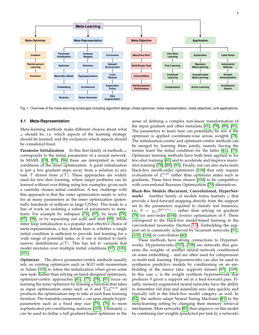
Fig. 1. Overview of the meta-learning landscape including algorithm design (meta-optimizer, meta-representation, meta-objective), and applications.
4.1 Meta-Representation
Meta-learning methods make different choices about what
ω should be, i.e. which aspects of the learning strategy
should be learned; and (by exclusion) which aspects should
be considered fixed.
Parameter Initialization
In this first family of methods ω
corresponds to the initial parameters of a neural network.
In MAML [19], [95], [96] these are interpreted as initial
conditions of the inner optimization. A good initialization
is just a few gradient steps away from a solution to any
task T drawn from p(T ). These approaches are widely
used for few-shot learning, where target problems can be
learned without over-fitting using few examples, given such
a carefully chosen initial condition. A key challenge with
this approach is that the outer optimization needs to solve
for as many parameters as the inner optimization (poten-
tially hundreds of millions in large CNNs). This leads to a
line of work on isolating a subset of parameters to meta-
learn. For example by subspace [74], [97], by layer [79],
[97], [98], or by separating out scale and shift [99]. While
inner loop initialization is a popular and effective choice of
meta-representation, a key debate here is whether a single
initial condition is sufficient to provide fast learning for a
wide range of potential tasks, or if one is limited to fairly
narrow distributions p(T ). This has led to variants that
model mixtures over multiple initial conditions [97], [100],
[101].
Optimizer
The above parameter-centric methods usually
rely on existing optimizers such as SGD with momentum
or Adam [102] to refine the initialization when given some
new task. Rather than relying on hand-designed optimizers,
optimizer-centric approaches [41], [77], [78], [91] focus on
learning the inner optimizer by training a function that takes
as input optimization states such as θ and ∇θLtask and
produces the optimization step to take at each base learning
iteration. The trainable component ω can span simple hyper-
parameters such as a fixed step size [75], [76] to more
sophisticated pre-conditioning matrices [103]. Ultimately ω
can be used to define a full gradient-based optimizer in the
sense of defining a complex non-linear transformation of
the input gradient and other metadata [41], [78], [89], [91].
The parameters to learn here can potentially be few if the
optimizer is applied coordinate-wise across weights [78].
The initialization-centric and optimizer-centric methods can
be merged by learning them jointly, namely having the
former learn the initial condition for the latter [41], [75].
Optimizer learning methods have both been applied to for
few-shot learning [41] and to accelerate and improve many-
shot learning [78], [89], [91]. Finally, one can also meta-learn
black-box zeroth-order optimizers [104] that only require
evaluations of Ltask rather than optimizer states such as
gradients. These have been shown [104] to be competitive
with conventional Bayesian Optimization [70] alternatives.
Black-Box Models (Recurrent, Convolutional, HyperNet-
work) Another family of models trains learners ω that
provide a feed-forward mapping directly from the support
set to the parameters required to classify test instances,
i.e., θ = gω(Dtrain) – rather than relying on gradient
[78] (or zero-order [104]) iterative optimization of θ. These
correspond to the black-box model-based learning in the
conventional taxonomy (Section 3.1). Embedding the sup-
port set is commonly achieved by recurrent networks [51],
[105], [106] or convolution [40].
These methods have strong connections to Hypernet-
works. Hypernetworks [107], [108] are networks that gen-
erate the weights of another neural network conditioned
on some embedding – and are often used for compression
or multi-task learning. Hypernetworks can also be used to
synthesize predictive models by conditioning on an em-
bedding of the source (aka. support) dataset [97], [109].
In this case ω is the weight synthesis hypernetwork that
produces θ given a support set in a feed-forward pass. Fi-
nally, memory-augmented neural networks have the ability
to remember old data and assimilate new data quickly, and
typically fall in the black-box model category as well. In
[82], the authors adapt Neural Turing Machines [81] to the
meta-learning setting by changing their memory retrieval
mechanism. Meta networks [83] then improve on this model
by combining fast weights (predicted per task by a network)
Meta-LearningApplicationMeta-ObjectiveMeta-RepresentationMeta-OptimizerGradientReinforcementLearningEvolutionParameterInitializationOptimizerBlack-Box ModelEmbeddingInstanceWeightsAttentionHyperparametersArchitectureCurriculumDataset/EnvironmentLoss/RewardExplorationPolicyDataAugmentationMany/Few-ShotMulti/Single-TaskOnline/OfflineFew-ShotLearningFast LearningContinualLearningCompressionExplorationBayesianMeta-LearningUnsupervisedMeta-LearningActive LearningLabel NoiseAdversarialDefenseDomainGeneralizationArchitectureSearchNoise GeneratorModulesNet/AsymptoticPerformance�
and slow weights (trained with REINFORCE across tasks) to
access memory. We note that some methods implement both
model-based and initial-condition [97] or optimizer-centric
[98] meta-learning in a single framework.
Embedding Functions (Metric Learning) This category of
methods are inspired by metric-learning approaches in con-
ventional machine learning, and are therefore categorised
as such in the conventional taxonomy (Section 3.1). They
are mainly applied to few-shot learning. Here the meta-
optimization process learns an embedding network ω that
transforms raw inputs into a representation suitable for
recognition by simple similarity comparison between query
and support instances [20], [79], [86], [110] (e.g., with cosine
similarity or euclidean distance).
However, metric-learning methods can be seen to be a
special case of the feed-forward black-box models above.
This is clearly the case for methods that produce logits
based on inner product between the embeddings of support
and query images xs and xq as gT
ω (xq)gω(xs) [79], [110].
Here the support image generates weights to interpret the
query example, making it a special case of a BBM where the
‘hypernetwork’ generates a linear classifier for the query set.
Vanilla methods in this family have been further enhanced
by making the embedding task-conditional [98], [111] or
learning a more elaborate comparison metric [87], [88].
Losses and Auxiliary Tasks Analogously to the meta-
learning approach to optimizer design, these approaches
(·) for the base model.
aim to learn the inner task-loss Ltask
Loss-learning approaches typically define a small neural
network that inputs quantities that are typically inputs to
losses (e.g., predictions, features, or model parameters) and
outputs a scalar to be treated as a loss by the inner (task)
optimizer. This has potential benefits such as leading to a
learned loss that is easier to optimize (e.g., less local minima)
than commonly used ones [23], [112], [113], leads to faster
learning with improved generalization [45], [114], [115], or
one whose minima correspond to a model more robust to
domain shift [44]. Furthermore, loss learning methods have
also been used to learn to learn from unlabeled instances
[98], [116]. Other applications include learning Ltask
() as
a differentiable approximation to a true non-differentiable
task loss such as area under precision recall curve [117],
[118].
ω
ω
Loss learning also arises in generalizations of self-
supervised [119], [120] or auxiliary task [121] learning.
In these problems unsupervised predictive tasks (such as
colourising pixels in vision [119], or simply changing pixels
in RL [121]) are defined and optimized in a multi-task
manner with the main task, but with the aim of improving
the representation in support of the main task. In this
case the best auxiliary task (loss) to use can be hard to
predict in advance, so meta-learning can be used to select
among several auxiliary losses according to their impact on
improving main task learning. I.e., ω is a per-auxiliary task
weight [68]. More generally, one can meta-learn an auxiliary
task generator that annotates examples with auxiliary labels
for the main multi-task model to predict [122].
Architectures Architecture discovery has always been an
important area in neural networks [39], [123], and one that
is not amenable to simple exhaustive search. Meta-Learning
7
can be used to automate this very expensive process by
learning architectures. Early attempts use RL and LSTMs to
learn to generate a description for a good architecture [28].
Evolutionary Algorithms [27] were also used in an attempt
to learn blocks within architectures modelled as graphs
which could mutate by editing their graph. Gradient-based
architecture representations have also been visited in the
form of DARTS [26] where the forward pass during training
consists in a softmax across the outputs of all possible layers
in a given block, which are weighted by coefficients to be
meta learned (i.e. ω). During meta-test, the architecture is
discretized by only keeping the layers corresponding to the
highest coefficients. The coefficients are learned greedily by
alternating a single inner step and a single outer step to
update architecture coefficients and network weights. Since
DARTS is still relatively slow and of limited accuracy, recent
efforts have focused on making architecture learning more
efficient through better differentiable approximations [124],
learning easy to adapt initializations [125], or architecture
priors [126]. More details on neural architecture search can
be found in Section 5.4.
Attention Modules
Attention mechanisms have been
shown to improve generalization performance and inter-
pretability. Such mechanisms have also formed part of the
meta-representation of various meta-learning models. For
example, they have been used as comparators of support
and target set items for metric-based transductive meta-
learners [127], as well as feature extractors to prevent
catastrophic forgetting in few-shot continual learning [128].
More recently, attention was also used to summarize the
distribution of an incoming text classification task [129].
Modules Modular meta-learning [130], [131] assumes that
the task agnostic knowledge ω defines a set of modules,
which are re-composed in a task specific manner defined by
θ in order to solve each encountered task. These strategies
can be seen as meta-learning generalizations of the typical
structural approaches to knowledge sharing that are well
studied in multi-task and transfer learning [65], [66], [132].
Hyper-parameters
In these methods ω includes hyperpa-
rameters of the base learning algorithm such as regulariza-
tion strength [25], per-parameter regularization [92], task-
relatedness in multi-task learning [67], or sparsity strength
in data cleansing [67]. Note that hyperparameters such
as step size and direction [75], [76] can be seen as part
of definition of the optimizer, and as such leads to an
overlap between hyper-parameter and optimizer learning
categories.
Data Augmentation
In supervised learning it is common
to improve generalization by synthesizing more training
data through label-preserving transformations on the ex-
isting data. The data augmentation operation is wrapped
up in optimization steps of the inner problem Eq. 6, and
is conventionally hand-designed. However, when ω defines
the data augmentation strategy, it can be learned by the
outer optimization in Eq. 5 in order to maximize validation
performance [133]. Since augmentation operations are typi-
cally non-differentiable, this requires reinforcement learning
[133], discrete gradient-estimators [134], or evolutionary
[135] methods. An open question is whether powerful GAN-
based data augmentation methods [136] can be used in
�
inner-level learning and optimized in outer-level learning.
Minibatch Selection, Sample Weights, and Curriculum
Learning When the base algorithm is minibatch-based
stochastic gradient descent, a design parameter of the
learning strategy is the batch selection process. Various
hand-designed methods [137] exist to improve on classic
randomly-sampled minibatches. Meta-learning approaches
to mini-batch selection define ω as an instance selection
probability [138] or small neural network that picks or
excludes instances [139] for inclusion in the next minibatch,
while the meta-loss can be defined as the learning progress
of the base model given the defined mini-batch selector.
Such selection methods can also provide a way to auto-
mate the learning of a curriculum. In conventional machine
learning, curricula are sequences of data or concepts to learn
that are hand-designed to produce better performance than
learning items in a random order [140], for instance by
focusing on instances of the right difficulty while rejecting
too hard or too easy (already learned) instances. Meta-
learning has the potential to automate this process and select
examples of the right difficulty by defining the teaching
policy as the meta-knowledge and training it to optimize
the progress of the student [139], [141].
and Environments
Related to mini-batch selection policies are methods that
learn per-sample loss weights ω for the training set [142],
[143]. This can be used to learn under label-noise by dis-
counting noisy samples [142], [143], discount outliers [67],
or correct for class imbalance [142].
Datasets, Labels
the
strangest choice of meta-representation is the support
dataset itself. This departs from our initial formalization
of meta-learning which considers the source datasets to
be fixed (Section 2.1, Eqs. 2-3). However, it can be easily
understood in the bilevel view of Eqs. 5-6. If the validation
set in the upper optimization is real and fixed, and a train
set in the lower optimization is paramaterized by ω, the
training dataset can be tuned by meta-learning to optimize
validation performance.
Perhaps
In dataset distillation [144], [145], the support images
themselves are learned such that a few steps on them
allows for good generalization on real query images. This
can be used to summarize large datasets into a handful
of images, which is useful for replay in continual learning
where streaming datasets cannot be stored.
Rather than learning the input images x for fixed labels
y, one can also learn the input labels y for fixed images x.
This can be used in semi-supervised learning, for example
to directly learn the unlabeled set’s labels to optimize vali-
dation set performance [146], or to train a label generation
function [147].
In the case of sim2real learning [148] in computer vision
or reinforcement learning, one uses an environment sim-
ulator to generate data for training. In this case one can
also train the graphics engine [149] or simulator [150] so
as to optimize the real-data (validation) performance of the
downstream model after training on data generated by that
environment simulator.
Discussion: Transductive Representations and Methods
Most of the representations ω discussed above are param-
eter vectors of functions that process or generate data.
8
However a few of the representations mentioned are trans-
ductive in the sense that the ω literally corresponds to data
points [144], labels [146], or per-sample weights [142]. This
means that the number of parameters in ω to meta-learn
scales as the size of the dataset. While the success of these
methods is a testament to the capabilities of contemporary
meta-learning [145], this property may ultimately limit their
scalability.
Distinct from a transductive representation are methods
that are transductive in the sense that they are designed to
operate on the query instances as well as support instances
[98], [122].
Discussion: Interpretable Symbolic Representations A
cross-cutting distinction that can be made across many of
the meta-representations discussed above is between unin-
terpretable (sub-symbolic) and human interpretable (sym-
bolic) representations. Sub-symbolic representations such
as when ω parameterizes a neural network [78], are more
commonly studied and make up the majority of studies
cited above. However, meta-learning with symbolic rep-
resentations is also possible, where ω represents symbolic
functions that are human readable as a piece of program
code [89], comparable to Adam [102]. Rather than neural
loss functions [44], one can train symbolic losses ω that are
defined by an expression comparable to cross-entropy [115].
One can also meta-learn new symbolic activations [151]
that outperform standards such as ReLU. As these meta-
representations are non-smooth, the meta-objective is non-
differentiable and is harder to optimize (see Section 4.2).
So the upper optimization for ω typically uses RL [89] or
evolutionary algorithms [115]. However, symbolic represen-
tations may have an advantage [89], [115], [151] in their
ability to generalize across task families. I.e., to span wider
distributions p(T ) with a single ω during meta-training, or
to have the learned ω generalize to an out of distribution
task during meta-testing (see Section 6).
4.2 Meta-Optimizer
Given a choice of which facet of the learning strategy to
optimize (as summarised above), the next axis of meta-
learner design is actual outer (meta) optimization strategy
to use for tuning ω.
Gradient A large family of methods use gradient descent
on the meta parameters ω [19], [41], [44], [67]. This requires
computing derivatives dLmeta/dω of the outer objective,
which are typically connected via the chain rule to the model
parameter θ, dLmeta/dω = (dLmeta/dθ)(dθ/dω). These
methods are potentially the most efficient as they exploit an-
alytical gradients of ω. However key challenges include: (i)
Efficiently differentiating through long computation graphs
where the inner optimization uses many steps, for example
through careful design of auto-differentiation algorithms
[25], [178] and implicit differentiation [145], [153], [179],
and dealing tractably with the required second-order gradi-
ents [180]. (ii) Reducing the inevitable gradient degradation
problems whose severity increases with the number of inner
loop optimization steps. (iii) Calculating gradients when
the base learner, ω, or Ltask include discrete or other non-
differentiable operations.
�


 2023年江西萍乡中考道德与法治真题及答案.doc
 2012年重庆南川中考生物真题及答案.doc
 2013年江西师范大学地理学综合及文艺理论基础考研真题.doc
 2020年四川甘孜小升初语文真题及答案I卷.doc
 2020年注册岩土工程师专业基础考试真题及答案.doc
 2023-2024学年福建省厦门市九年级上学期数学月考试题及答案.doc
 2021-2022学年辽宁省沈阳市大东区九年级上学期语文期末试题及答案.doc
 2022-2023学年北京东城区初三第一学期物理期末试卷及答案.doc
 2018上半年江西教师资格初中地理学科知识与教学能力真题及答案.doc
 2012年河北国家公务员申论考试真题及答案-省级.doc
 2020-2021学年江苏省扬州市江都区邵樊片九年级上学期数学第一次质量检测试题及答案.doc
 2022下半年黑龙江教师资格证中学综合素质真题及答案.doc