Constrained Local Graph Clustering by Colored Random Walk
Yaowei Yan
yxy230@ist.psu.edu
Pennsylvania State University
Yuchen Bian
yub31@ist.psu.edu
Pennsylvania State University
Dongsheng Luo
dul262@ist.psu.edu
Pennsylvania State University
Dongwon Lee
dlee@ist.psu.edu
Pennsylvania State University
ABSTRACT
Detecting local graph clusters is an important problem in big graph
analysis. Given seed nodes in a graph, local clustering aims at find-
ing subgraphs around the seed nodes, which consist of nodes highly
relevant to the seed nodes. However, existing local clustering meth-
ods either allow only a single seed node, or assume all seed nodes
are from the same cluster, which is not true in many real applica-
tions. Moreover, the assumption that all seed nodes are in a single
cluster fails to use the crucial information of relations between seed
nodes. In this paper, we propose a method to take advantage of such
relationship. With prior knowledge of the community membership
of the seed nodes, the method labels seed nodes in the same (differ-
ent) community by the same (different) color. To further use this
information, we introduce a color-based random walk mechanism,
where colors are propagated from the seed nodes to every node in
the graph. By the interaction of identical and distinct colors, we can
enclose the supervision of seed nodes into the random walk process.
We also propose a heuristic strategy to speed up the algorithm by
more than 2 orders of magnitude. Experimental evaluations reveal
that our clustering method outperforms state-of-the-art approaches
by a large margin.
CCS CONCEPTS
• Mathematics of computing → Graph algorithms; • Infor-
mation systems → Clustering; • Theory of computation →
Random walks and Markov chains.
KEYWORDS
community detection; local graph clustering; random walk; non-
Markovian
ACM Reference Format:
Yaowei Yan, Yuchen Bian, Dongsheng Luo, Dongwon Lee, and Xiang Zhang.
2019. Constrained Local Graph Clustering by Colored Random Walk. In
Proceedings of the 2019 World Wide Web Conference (WWW ’19), May 13–17,
2019, San Francisco, CA, USA. ACM, New York, NY, USA, 10 pages. https:
//doi.org/10.1145/3308558.3313719
This paper is published under the Creative Commons Attribution 4.0 International
(CC-BY 4.0) license. Authors reserve their rights to disseminate the work on their
personal and corporate Web sites with the appropriate attribution.
WWW ’19, May 13–17, 2019, San Francisco, CA, USA
© 2019 IW3C2 (International World Wide Web Conference Committee), published
under Creative Commons CC-BY 4.0 License.
ACM ISBN 978-1-4503-6674-8/19/05.
https://doi.org/10.1145/3308558.3313719
Xiang Zhang
xzhang@ist.psu.edu
Pennsylvania State University
Community returned by seed 1
Hong Cheng Xiaofei He
Xifeng Yan
Ke Wang
Seed 2
H. Kitagawa
I. Kamel
Jiawei Han
Wei Wang
Papadimitriou
C. Faloutsos
Xiaoxin YinH. Gonzalez
Jimeng Sun C.Traina Jr.
Flip Korn
H. Jagadish
Seed 1
Community returned by both seed 1 and 2
Community returned by seed 2
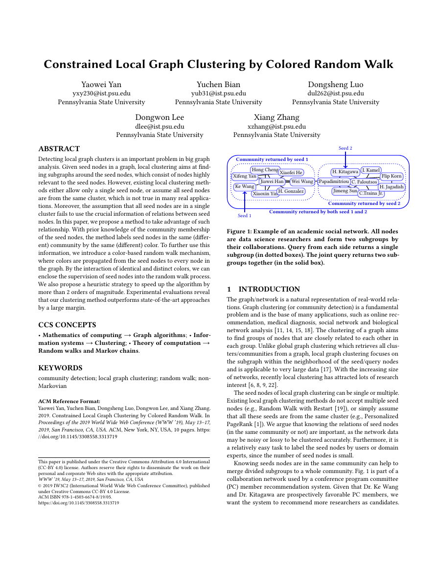
Figure 1: Example of an academic social network. All nodes
are data science researchers and form two subgroups by
their collaborations. Query from each side returns a single
subgroup (in dotted boxes). The joint query returns two sub-
groups together (in the solid box).
1 INTRODUCTION
The graph/network is a natural representation of real-world rela-
tions. Graph clustering (or community detection) is a fundamental
problem and is the base of many applications, such as online rec-
ommendation, medical diagnosis, social network and biological
network analysis [11, 14, 15, 18]. The clustering of a graph aims
to find groups of nodes that are closely related to each other in
each group. Unlike global graph clustering which retrieves all clus-
ters/communities from a graph, local graph clustering focuses on
the subgraph within the neighborhood of the seed/query nodes
and is applicable to very large data [17]. With the increasing size
of networks, recently local clustering has attracted lots of research
interest [6, 8, 9, 22].
The seed nodes of local graph clustering can be single or multiple.
Existing local graph clustering methods do not accept multiple seed
nodes (e.g., Random Walk with Restart [19]), or simply assume
that all these seeds are from the same cluster (e.g., Personalized
PageRank [1]). We argue that knowing the relations of seed nodes
(in the same community or not) are important, as the network data
may be noisy or lossy to be clustered accurately. Furthermore, it is
a relatively easy task to label the seed nodes by users or domain
experts, since the number of seed nodes is small.
Knowing seeds nodes are in the same community can help to
merge divided subgroups to a whole community. Fig. 1 is part of a
collaboration network used by a conference program committee
(PC) member recommendation system. Given that Dr. Ke Wang
and Dr. Kitagawa are prospectively favorable PC members, we
want the system to recommend more researchers as candidates.
�
Clustering if seeds 1 and 2 are different
Seed 2
Polyps
Benign diseases
Seed 1
Cancers
Clustering if seed 1 and 2 are similar
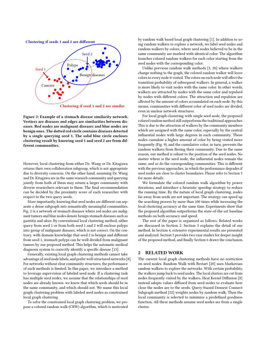
Figure 2: Example of a stomach disease similarity network.
Vertices are diseases and edges are similarities between dis-
eases. Red nodes are malignant diseases and blue nodes are
benign ones. The dotted red circle contains diseases detected
by a single querying seed 1. The solid blue circle encloses
clustering result by knowing seed 1 and seed 2 are from dif-
ferent communities.
However, local clustering from either Dr. Wang or Dr. Kitagawa
returns their own collaboration subgroup, which is not appropriate
due to diversity concerns. On the other hand, assuming Dr. Wang
and Dr. Kitagawa are in the same research community and querying
jointly from both of them may return a larger community with
diverse researchers relevant to them. The final recommendation
can be decided by the proximity score of each researcher with
respect to the two query seeds.
More importantly, knowing that seed nodes are different can sep-
arate a dense subgraph into semantically meaningful communities.
Fig. 2 is a network of stomach diseases where red nodes are malig-
nant tumors and blue nodes denote benign stomach diseases such as
gastritis and ulcer. By conventional local clustering method, either
query from seed 1 or from both seed 1 and 2 will enclose polyps
into group of malignant diseases, which is not correct. On the con-
trary, with domain knowledge that seed 2 is benign and different
from seed 1, stomach polyps can be well divided from malignant
tumors by our proposed method. This helps the automatic medical
diagnosis system to correctly identify a specific disease [13].
Generally, existing local graph clustering methods cannot take
advantage of seed node labels, and prefer well-structured networks [8].
For networks without clear community structures, the performance
of such methods is limited. In this paper, we introduce a method
to leverage supervision of labeled seed node. If a clustering task
has multiple seed nodes, we assume that the relationships of seed
nodes are already known: we know that which seeds should be in
the same community, and which should not. We name this local
graph clustering problem with labeled seed nodes as constrained
local graph clustering.
To solve the constrained local graph clustering problem, we pro-
pose a colored random walk (CRW) algorithm, which is motivated
by random walk based local graph clustering [1]. In addition to us-
ing random walkers to explore a network, we label seed nodes and
random walkers by colors, where seed nodes believed to be in the
same community are marked with identical color. The algorithm
launches colored random walkers for each color starting from the
seed nodes with the corresponding color.
Unlike previous random walk methods [3, 20] where walkers
change nothing to the graph, the colored random walker will leave
colors to every node it visited. The colors on each node will affect the
transition probability of subsequent walkers. In general, a walker
is more likely to visit nodes with the same color. In other words,
walkers are attracted by nodes with the same color and repulsed
by nodes with different colors. The attraction and repulsion are
affected by the amount of colors accumulated on each node. By this
means, communities with different color of seed nodes are divided,
even in unclear network structures.
For local graph clustering with single seed node, the proposed
colored random method still outperforms the traditional approaches.
This is due to the attraction of walkers by the community members
which are assigned with the same color, especially by the central
influential nodes with large degrees in each community. These
nodes cumulate a higher amount of color by being visited more
frequently (Fig. 9), and the cumulative color, in turn, prevents the
random walkers from fleeing their community. Due to the same
reason, our method is robust to the position of the seed nodes. No
matter where is the seed node, the influential nodes remain the
same, and so do the corresponding communities. This is different
with the previous approaches, in which the performance degrades if
seed nodes are close to cluster boundaries. Please refer to Section 5
for more details.
We formulate the colored random walk algorithm by power
iterations, and introduce a heuristic speedup strategy to reduce
the running time. By the nature of local graph clustering, nodes
far away from seeds are not important. The strategy can speed up
the searching process by more than 100 times while increasing the
local clustering accuracy at the same time. Experiments show that
the proposed algorithm outperforms the state-of-the-art baseline
methods on both accuracy and speed.
The rest of the paper is organized as follows. Related works
are discussed in Section 2. Section 3 explains the detail of our
method. In Section 4, extensive experimental results are presented
and analyzed. Section 5 provides two case studies for deeper insight
of the proposed method, and finally Section 6 draws the conclusion.
2 RELATED WORK
The current local graph clustering methods have no restriction
on seed nodes. Random Walk with Restart [20] uses Markovian
random walkers to explore the networks. With certain probability,
the walkers jump back to seed nodes. The local clusters are cut from
nodes frequently visited by the walkers. Heat Kernel Diffusion [8]
instead adopts values diffused from seed nodes to evaluate how
close the nodes are to the seeds. Query-biased Densest Connect
Subgraph method [22] weights nodes by random walk. Then the
local community is selected to minimize a predefined goodness
function. All these methods assume seed nodes are from a single
cluster.
-4-3-2-101234-4-3-2-101234 �
Semi-supervised learning, including semi-supervised cluster-
ing with constrains, gained success as they do not require a large
amount of human annotations [4]. In semi-supervised learning, the
labels are propagated from labeled seed instances by random-walk-
like mechanisms through the similarity graph, and then a classifier
is trained to categorize all other instances [24, 25]. However, tradi-
tional semi-supervised learning focuses more on classification than
clustering, and is a heavy framework since it considers both local
and global consistency during the learning process.
The colored random walk is also relevant to the Vertex-reinforced
Random Walk (VRW), which views graph nodes as urns [16]. Each
time the random walker visits a node, it puts a ball with its color
into the corresponding urn. The further visiting probability of the
random walker is reinforced by the numbers and colors of balls in
each node. Though it is proved that single-color VRW is guaranteed
to converge to a distribution [2], the converged distribution is not
unique due to the randomness of the walker, which diminishes
the performance of VRW in local graph clustering. Moreover, the
theories of multi-color VRW are still underdeveloped.
3 OUR PROPOSAL
Local graph clustering requires proximity measurement to decide
which nodes should be in a local cluster. Random walk based ap-
proaches such as Random Walk with Restart (a.k.a. Personalized
PageRank) are commonly used to evaluate the node proximity in
graphs [20]. Compared with other methods, random walk takes
advantage of local network structure and reports better perfor-
mance [9]. In this work, we extend the random walk method to
colored random walk to solve the problem of local graph clustering
with constrains.
transition matrix with entries Pji = Aij /
3.1 Preliminaries
The local graph clustering targets on a graph G = (V , E), where
V is the node set and E is the edge set. The adjacency matrix of
graph G is denoted by A, whose element Aij is the edge weight
between node Vi and node Vj. P is the transposed column-stochastic
j Aij. The main symbols
and their definitions can be found in Table 1.
The core function of local graph clustering is to measure the
proximity of each node with the seed node(s). In Random Walk
with Restart (RWR), a random walker starts from the seed node q,
and randomly walks to a neighbor node according to edge weights.
At each time point (t + 1), the walker continues walking with
probability α or returns to the query node q with probability (1−α ).
The proximity score of node p with respect to node q is defined as
the converged probability that the walker visits node p:
c(t +1) = α · P · c(t ) + (1 − α ) · s
(1)
th
where s is the column vector of the initial distribution with q
entry as 1 and all other entries 0, and c is the current distribution
vector whose p
th entry is the visiting probability of node p.
RWR can be extended to accommodate multiple seed nodes. For n
seed nodes, the initial vector s consists of entries with value 1/n for
each seed node. However, if seed nodes are from multiple clusters,
RWR cannot use such information. One may run RWR multiple
times, each for a single seed node, yet this approach fails to take full
Table 1: Main symbols
Symbol
G = (V , E)
A, P
c, s
α, θ
ψ (t )
λ1, λ2
Definition
graph G with node set V and edge set E
adjacency matrix and transition matrix
current and initial color distributions
forward probability and color threshold
decaying factor at time t
attraction and repulsion coefficient
advantage the prior knowledge of cluster membership of the seed
nodes. For example, if two seed nodes are known from different
clusters, walkers of each seed node should avoid walking into the
other seed’s cluster. We give the formal definition of constrained
local graph clustering as follows.
Definition 3.1 (Constrained local graph clustering). Given graph
G = (V , E) and seed node set with K different colors, the con-
strained local graph clustering aims to find K local communities
containing seed nodes of each color.
3.2 The Colored Random Walk
To solve the constrained local graph clustering problem, we propose
a Colored Random Walk (CRW) method in this section, which takes
advantage of seed node labels. Seed nodes of the same cluster are
assigned with identical color, and seed nodes from different clusters
have different colors. For each color, the algorithm sends out a
colored walker from the corresponding seed nodes to explore the
network. During the exploration, the walker leaves a certain amount
of colored values to the visited nodes, similar to the RWR method
in Eq. 1.
The main difference between CRW and conventional RWR is that
the movement of walkers is affected by existing colors of nodes.
Generally, a walker is more likely to visit nodes with identical
colors, and is less likely to visit nodes with distinct colors. Since
color values are changed at each time point t, the transition matrix
P should be updated accordingly.
For a constrained local graph clustering task with K colors, the
CRW algorithm maintains K transition matrix P(k,t ) for color k at
time t. Then the Eq. 1 expands to a new power iteration formula
(2)
where c(k,t ) is the distribution of color k at time t, and s(k ) is the
initial vector of color k, respectively.
c(k,t +1) = α · P(k,t ) · c(k,t ) + (1 − α ) · s(k )
3.3 Transition Matrix Reinforcement
The transition matrix P(k,t ) in Eq. 2 is based on the original transi-
tion matrix P, and is reinforced by all current color distributions
c(ℓ,t ), 1 ≤ ℓ ≤ K. The reinforcement is done by
P(k,t ) = P ◦ (1 + R(k,t ) )
(3)
where operator ◦ is the Hadamard (entry-wise) product of two
matrices with the same size [7]. By Hadamard product, we avoid
adding new edges to graph G, and the reinforcement is done by
weight adjustment of existing edges. In the Eq. 3, ‘1’ is used to keep
the original transition matrix P as part of the reinforced transition
�
λ1
−λ2
ℓ
matrix P(k,t ). R is a coefficient matrix defined by its entry
R(k,t )
ij
=
c(ℓ,t )
i
· λk ℓ,
λk ℓ =
k = ℓ
k ℓ
(4)
In Eq. 4, if the factor λk ℓ is defined as positive when color k
equals color ℓ, and negative otherwise. This definition increases the
likelihood of a walker going to the node with identical color, and
decreases the likelihood of walking to the node with different colors.
The mechanism can be understood as that, a walker is attracted by
nodes with the same color, and repulsed by nodes with different
colors. Here we denote by λ1 the attraction coefficient and by λ2
the repulsion coefficient.
ij ← 0 if P(k,t )
/
ij ← P(k,t )
By Eq. 3 and 4, the entries of P(k,t ) are possibly negative. To make
P(k,t ) as a transition matrix meaningful, it is normalized before used
in Eq. 2. The normalization includes two parts. First, the negative
entries of P(k,t ) are set to be zero: P(k,t )
< 0, and
then each entry of the matrix is divided by the sum of its column
to make the matrix column stochastic: P(k,t )
.
i P(k,t )
3.4 Convergence
Unlike the traditional random walk methods which have stationary
transition matrix P, the transition matrix P(k,t ) of colored random
walk varies at each time t. To guarantee the convergence of Eq. 2, we
introduce a decaying mechanism changing P(k,t ) to P(k,t ) (Eq. 5),
where the value of function ψ (t ) approaches to 0 when t increases.
Then the colored random walk is adapted to Eq. 6.
ij
ij
ij
P(k,t ) =
ψ (t ) · P(k,t ) + (1 − ψ (t )) · P(k,t−1)
t = 0
t ≥ 1
(5)
c(k,t +1) = α · P(k,t ) · c(k,t ) + (1 − α ) · s(k )
(6)
Here the definition of P remains the same with Eq. 3 and Eq. 4.
Intuitively, when ψ (t ) → 0, Pk,t → Pk,t−1, meaning that Pk,t
converges. With a converged Pk,t , the proximity score vector c(k,t )
converges, similar to the conventional random walk. The formal
proof of convergence of c(k,t ) is given by Theorem 3.2.
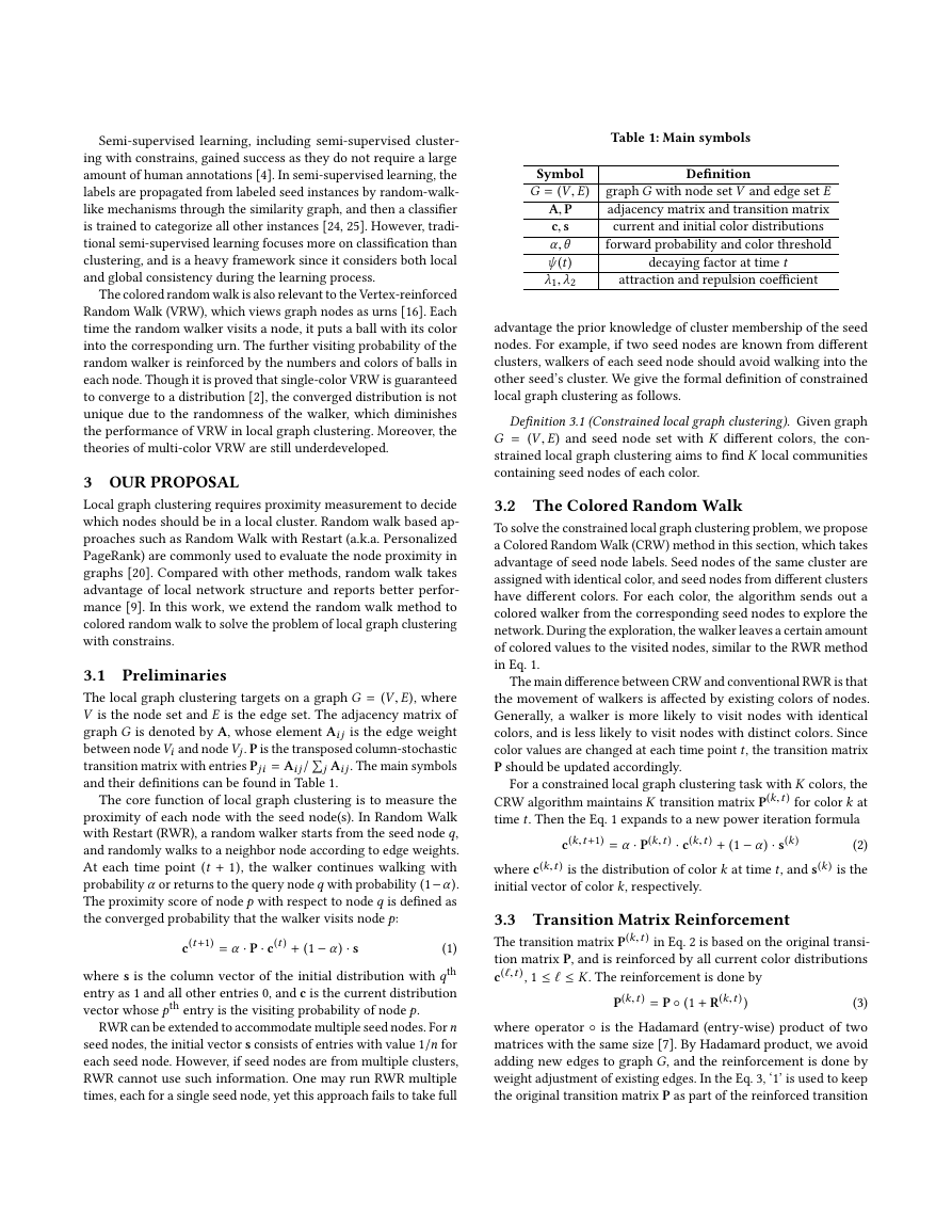
Theorem 3.2 (Convergence of colored random walk). Both
P(k,t ) and c(k,t ) in Eq. 5 and Eq. 6 converge if ψ (t ) = Ω(αt ).
Proof. To ease the description, we combine distributions, rein-
forced transition matrices, and initial vectors of all color at time t
by
c(K,t )
c(t ) =
P(2,t )
P(1,t )
c(1,t )
c(2,t )
...
s(1)
s(2)
...
s(K )
Evidently, Eq. 7 equals to Eq. 6 for all color 1 ≤ k ≤ K. Similarly
we define P(t ) as diagonal combination of all P(t,k ).
c(t +1) = α · P(t ) · c(t ) + (1 − α ) · s
(7)
For convergence of decayed transition matrix P(t ), it is easy to
P(K,t )
. . .
0
, P(t ) =
0
, s =
know that for t ≥ 1,
∥P(t ) − P(t−1)∥1 = ψ (t )∥P(t ) − P(t−1)∥1 ≤ 2ψ (t )
P
:P, S, α, λ1, λ2, T , ψ (t )
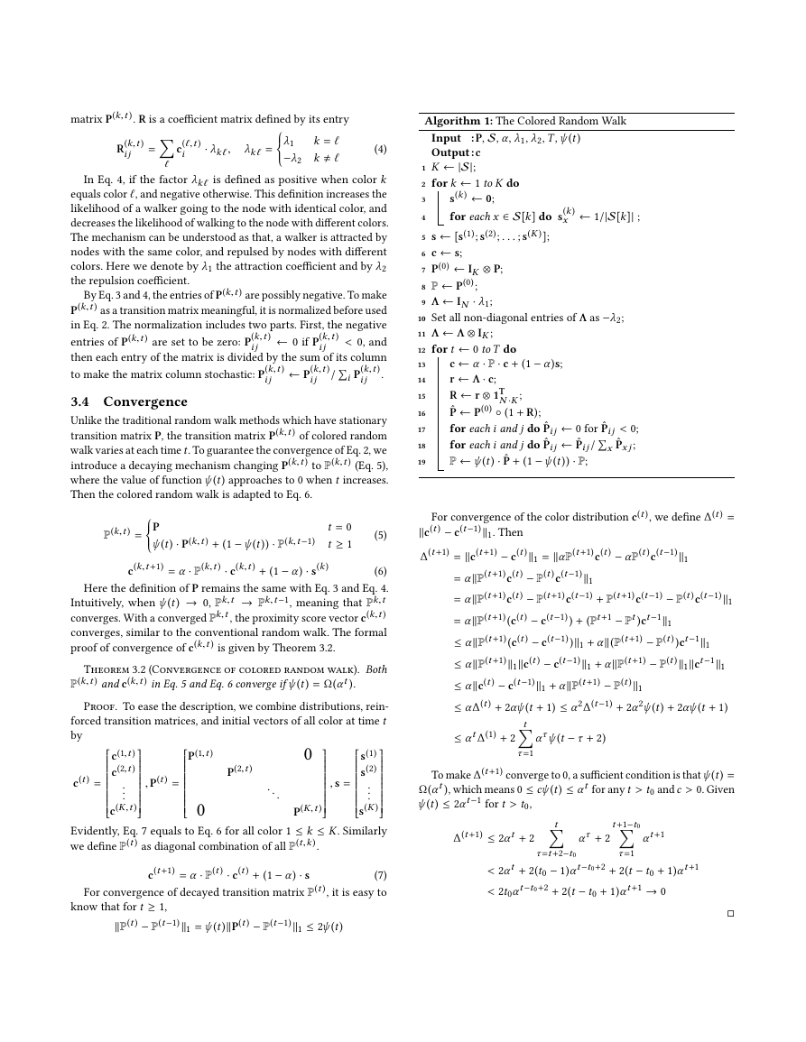
Algorithm 1: The Colored Random Walk
Input
Output:c
1 K ← |S|;
2 for k ← 1 to K do
s(k ) ← 0;
for each x ∈ S[k] do s(k )
3
4
x ← 1/|S[k]| ;
5 s ← [s(1); s(2); . . . ; s(K )];
6 c ← s;
7 P(0) ← IK ⊗ P;
8 P ← P(0);
9 Λ ← IN · λ1;
10 Set all non-diagonal entries of Λ as −λ2;
11 Λ ← Λ ⊗ IK ;
12 for t ← 0 to T do
;
N ·K
c ← α · P · c + (1 − α )s;
r ← Λ · c;
R ← r ⊗ 1T
ˆP ← P(0) ◦ (1 + R);
for each i and j do ˆPij ← 0 for ˆPij < 0;
ˆPx j;
P ← ψ (t ) · ˆP + (1 − ψ (t )) · P;
for each i and j do ˆPij ← ˆPij /
x
13
14
15
16
17
18
19
For convergence of the color distribution c(t ), we define ∆(t ) =
∥c(t ) − c(t−1)∥1. Then
∆(t +1) = ∥c(t +1) − c(t )∥1 = ∥α P(t +1)c(t ) − α P(t )c(t−1)∥1
= α∥P(t +1)c(t ) − P(t )c(t−1)∥1
= α∥P(t +1)c(t ) − P(t +1)c(t−1) + P(t +1)c(t−1) − P(t )c(t−1)∥1
= α∥P(t +1) (c(t ) − c(t−1) ) + (Pt +1 − Pt )ct−1∥1
≤ α∥P(t +1) (c(t ) − c(t−1) )∥1 + α∥(P(t +1) − P(t ) )ct−1∥1
≤ α∥P(t +1)∥1∥c(t ) − c(t−1)∥1 + α∥P(t +1) − P(t )∥1∥ct−1∥1
≤ α∥c(t ) − c(t−1)∥1 + α∥P(t +1) − P(t )∥1
∆(t−1) + 2α
≤ α ∆(t ) + 2αψ (t + 1) ≤ α
2
ψ (t ) + 2αψ (t + 1)
≤ αt ∆(1) + 2
ατ ψ (t − τ + 2)
t
2
τ =1
To make ∆(t +1) converge to 0, a sufficient condition is thatψ (t ) =
Ω(αt ), which means 0 ≤ cψ (t ) ≤ αt for any t > t0 and c > 0. Given
ψ (t ) ≤ 2αt−1 for t > t0,
∆(t +1) ≤ 2αt + 2
ατ + 2
αt +1
t
τ =t +2−t0
t +1−t0
τ =1
< 2αt + 2(t0 − 1)αt−t0+2 + 2(t − t0 + 1)αt +1
< 2t0αt−t0+2 + 2(t − t0 + 1)αt +1 → 0
□
�
5
6
7
8
9
10
11
12
13
14
15
16
17
18
3.5 The Algorithm
By Eq. 7, we can formulate the colored random walk as shown in
Algorithm 1. The input of the algorithm includes original transition
matrix P, seed node sets S of all colors, penalty factor α, attraction
coefficient λ1 and repulsion coefficient λ2, together with the number
of iterations T and the decaying faction ψ (t ). The output of the
algorithm is the color distribution vector c for all colors. The details
of the algorithm are as follows.
Lines 1 – 11 initialize the algorithm. Specifically, in line 1 we
get the number of colors K by the number of seed node sets in
S. Lines 3 and 4 prepare for the initial color vectors s(k ) for each
color k. From line 5 to line 8 we combine initial distributions and
transition matrix of all colors together by s and P(0), as explained
in Section 3.4, and initialize the color distribution vector c and the
modified transition matrix P.
To calculate the color reinforcement for each node, we create a
N × N factor matrix Λ (lines 9 to 11), which originally has the value
of λ1 on all diagonal entries and−λ2 on all non-diagonal entries. The
size of matrix Λ is then amplified (line 11) by Kronecker Product [7]
with an identity matrix IK , to multiply with vector c (line 14), which
is a matrix-form equivalence to the operation in Eq. 4.
The for loop from line 12 to 19 is the power iteration process.
We first generate the color distribution for next iteration (line 13),
and then generate the reinforcement vector r (line 14). Vector r is
repeated to form a matrix R (line 15), which means that the rein-
forcement is fair to every node. After generating new reinforced
matrix ˆP (line 16), we remove negative entries (line 17) and nor-
malize it to column stochastic (line 18), and update the decayed
transition matrix for the next iteration (line 19).
The power iteration part of the algorithm is critical in analyzing
the time complexity, where all operations including calculations
of color distribution (line 13), reinforcement (line 14) and decayed
transition matrix (line 19) take O (K|E|), if we base the operations on
sparse matrices. Therefore, the overall time complexity is O (T K|E|).
As empirically reported in [9], T = 10 is sufficient for the conver-
gence of distribution c.
With the distribution c for each color, we rank nodes by their
colors and cut local communities by sweeping from the top-rank
node and find a cluster with minimum conductance [1].
3.6 Speedup Strategy
Time complexity of the proposed colored random walk algorithm is
proportional to the number of edges |E|, implying that the algorithm
searches the entire graph for local clusters. This is undesirable as
the task of local clustering focuses only on the nodes close to the
seeds.
In this section, we propose a localized variant of Algorithm 1,
with the basic idea that random walkers only search the influential
nodes around the seed nodes. Unlike Algorithm 1 where the walkers
go as far as T -hops from the seeds, we only consider nodes with
colors above a given tolerance threshold θ.
As the random process in Eq. 2 can be viewed as the diffusion of
colors from each node to its neighbors, the key point of Algorithm 2
is that only colors with values above a threshold θ will diffuse to
next iteration. The intuition behind this is that small color amount
will not affect colors of next iteration very much. When a walker
Algorithm 2: The Localized Colored Random Walk
Input
Output:c
:P, S, α, λ1, λ2, T , θ
1 for each color k do
2
c(k ) ← 0;
for each node i ∈ S[k] do c(k )
3
i ← 1/|S[k]| ;
4 for t ← 1 to T do
ˆc(k ) ← 0;
for each color k do
i > θ do
for each c(k )
p ← 0;
for each neighbor j of node i do
pj ← P(k,t )
for each color ℓ do
ij
;
if ℓ = k then pj ← pj + λ1 · c(ℓ)
else pj ← pj − λ2 · c(k )
;
j
;
j
· pj / p ;
+ α · c(k )
i
if pj < 0 then pj ← 0 ;
for each pj > 0 do ˆc(k )
j ← ˆc(k )
for each seed node i ∈ S[k] do
+ (1 − α )/|S[k]|;
i ← ˆc(k )
ˆc(k )
i
j
for each color k do c(k ) ← ˆc(k ) ;
reaches a node with color value less than θ, it stops there and does
not go to the node’s neighbors, which prevents the process from
searching too many further nodes. We also neglect the decaying
function ψ (t ) and reinforce the node on demand (with color value
greater than θ) to accelerate the algorithm.
In Algorithm 2, lines 1 – 3 initialize the color distribution accord-
ing to seed nodes, and lines 4 – 18 simulate the power iteration in
a heuristic way. In this heuristic algorithm, we remove the process
of decaying, as it is shown that the result of experiments without
decaying is similar. Specifically, at each iteration (line 4) the current
color scores are in c(k ) for color k, and the new scores for next iter-
ation are calculated and stored in ˆc(k ). Note that, c(k ) is changed
to ˆc(k ) after the scores of all colors are updated (line 18). Note that
the color scores are updated simultaneously.
By this strategy, though color values diminish at each iteration,
the summation of colors remains its majority value. The difference
turns out to be less than 1%.
4 EXPERIMENTAL VALIDATION
Extensive experiments are conducted on both synthetic and real-
world data to evaluate the effectiveness and efficiency of the pro-
posed algorithms. All experiments are performed on a server with
Redhat OS, Xeon 2.6GHz CPU, and 64G memory. The core functions
are implemented by C++.
Each experimental result is gathered on average of 10,000 trials.
The querying seeds are randomly selected. The accuracy is mea-
sured by F1-score, which is defined as 2pr /(p + r ), where p and r
�
are precision and recall, respectively.
Table 2: 1-query accuracy for non-overlapping clusters
4.1 Non-overlapping Clusters
We use the following networks with non-overlapping ground truth
clusters to test the effectiveness of our proposed method. The clus-
ters are large enough to test the searching ability of the colored
random algorithm algorithm.
Disease networks. The networks contain a disease similarity net-
work [13] with 9,721 diseases. For this network, there are two sets
of clustering ground truth for the disease network, with 17 classes
and 47 classes, respectively. We use both sets of ground truth, and
denote the experiments by Disease 1 and Disease 2, accordingly.
Disease 3 is a phenotype similarity network with 5,080 diseases in
20 categories [21].
Gene network. The gene network represents the functional rela-
tionship between 8,503 genes [21] with 200 pathway labels.
Author network. This network comprises 20,111 authors from
4 research areas: Data Mining, Data Base, Information Retrieval
and Machine Learning. The edge of this network is the number of
papers co-published by the authors.
Conference network. This is a full graph comprises 20 main con-
ferences from the same 4 areas with the author network. The edges
are cosine similarity of keywords from the publication of the con-
ferences. We use research areas as the ground truth for both author
network and conference network.
Since no previous method is designed for the constrained local
graph clustering problem, we compare the proposed colored ran-
dom walk (CRW) method with the following five state-of-the-art
local clustering methods, which support multiple seed node query-
ing: Random Walk with Restart (RWR) [20] uses Eq. 1 to calculate
the proximity score of each node; Heat Kernel Diffusion (HKD) [8]
measures node proximity by heat kernel network diffusion; Query-
biased Densest Connect subgraph (QDC) [22] assigns weights to
nodes using RWR scores and finds the query biased densest sub-
graph; Vertex-reinforced Random Walk (VRW) [12] reinforces the
next-hop visiting probability by previous visiting counts. For our
method CRW, we use the localized colored random walk (Algo-
rithm 2) with α = 0.9, λ1 = 1000, λ2 = 10, θ = 10−5.
Effectiveness evaluations are conducted on the selected networks.
Since the accuracy difference between our two algorithms is small,
we present the results of Algorithm 2 only. Table 2 shows the result
of single seed node querying. By column “CRW” we only use one
seed node with a single color, so there is no repulsion of different
colors, which serves as a baseline of our method. From the results
in Table 2, it can be seen that even the basic CRW can outperform
the state-of-the-art methods in terms of clustering accuracy.
In Table 2 we add an extra column of CRW1
1, which randomly
picks up two seed nodes of different colors to examine the impact
of color repulsion. Comparison of CRW and CRW1
1 shows that
resistance of distinct colors helps to improve the clustering accuracy
significantly. On all datasets CRW1
1 achieves the best performance.
Table 3 shows the result of 2-seed-node query on the same 6
datasets. For each method except CWR2
2 we use two seed nodes
from the same cluster. CWR2
1 by choosing 2
colors, each having two seeds. Though initially VRW is not designed
2 is similar to CWR1
F1-score
Disease 1
Disease 2
Disease 3
Gene
Author
Conference
RWR HKD QDC VRW CRW CRW1
1
0.33
0.37
0.42
0.53
0.24
0.38
0.05
0.22
0.27
0.40
0.42
0.71
0.34
0.49
0.30
0.16
0.30
0.66
0.27
0.48
0.30
0.06
0.03
0.38
0.11
0.32
0.14
0.09
0.01
0.40
0.08
0.25
0.13
0.15
0.01
0.57
Table 3: 2-query accuracy for non-overlapping clusters
F1-score
Disease 1
Disease 2
Disease 3
Gene
Author
Conference
RWR HKD QDC VRW CRW CRW2
2
0.40
0.44
0.43
0.61
0.26
0.39
0.05
0.35
0.32
0.41
0.43
0.91
0.41
0.57
0.38
0.21
0.35
0.89
0.30
0.54
0.33
0.07
0.02
0.45
0.11
0.38
0.19
0.08
0.01
0.40
0.10
0.29
0.10
0.17
0.01
0.57
for multiple seed nodes, we make it work by adding extra random
walkers that are reinforced by rules of the original VRW. Comparing
Table 3 with Table 2, the conclusion is that almost all methods
improve clustering accuracy by having more seeds. Furthermore,
CWR gains more improvement on average. Again CRW1
1 and CRW2
2
have the best performance among all chosen methods.
4.2 Overlapping Clusters
Intuitively colored random walk works with non-overlapping clus-
ters. However, due to its color-agglomerating nature, it also works
for detecting overlapping clusters. Table 4 lists the statistics 4 of
networks with overlapping ground truth communities (Amazon,
DBLP, YouTube, LiveJournal). These datasets are publicly available
at http://snap.stanford.edu. For the quality of clusters, we select
clusters with size larger than 10, and within ±3σ range of the av-
erage cluster size. The last column of Table 4 shows the mean and
standard deviation (σ) of the chosen clusters.
Table 4: Networks with overlapping communities
Name
Amazon
DBLP
YouTube
LiveJournal
|V |
334,863
317,080
1,134,890
3,997,962
|E|
925,872
1,049,866
2,987,624
34,681,189
# clusters
75,149
13,477
8,385
287,512
avg (σ)
13.23 (11.24)
10.87 (20.41)
10.22 (18.81)
23.67 (24.75)
Table 5: 1-query accuracy on overlapping communities
F1-score
Amazon
DBLP
YouTube
LiveJournal
RWR HKD QDC VRW CRW CRW1
1
0.92
0.93
0.41
0.76
0.05
0.30
0.69
0.84
0.92
0.72
0.27
0.81
0.93
0.59
0.06
0.74
0.90
0.65
0.19
0.74
0.70
0.57
0.13
0.42
�
Table 6: 2-query accuracy on overlapping communities
F1-score
Amazon
DBLP
YouTube
LiveJournal
RWR HKD QDC VRW CRW CRW2
2
0.93
0.96
0.42
0.81
0.05
0.42
0.69
0.86
0.95
0.78
0.38
0.84
0.94
0.61
0.06
0.75
0.91
0.73
0.21
0.79
0.79
0.68
0.16
0.45
The clustering results are listed in both Table 5 and Table 6. It
shows that 2-seed quires are generally better than single seed node.
Among all methods HKD is relatively good since it is refined for
the small overlapping communities. However, more seed nodes do
not improve its performance very much (only 1% on average). The
probability-reinforced methods VRW and CRW gain the biggest
improvement by adding an extra seed. Once again our proposed
method leads the accuracy measurements. For seed nodes more
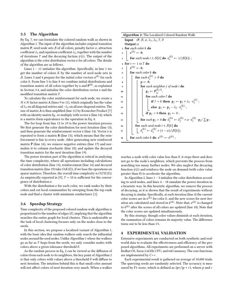
than 2, Fig. 3 shows that most methods perform better with more
seeds. However, CRW, VRW and QDC take better advantage of
more seed nodes, as they all have mechanisms of reinforcement on
node weights.
Fig. 3 gives the results where seed nodes are from a single commu-
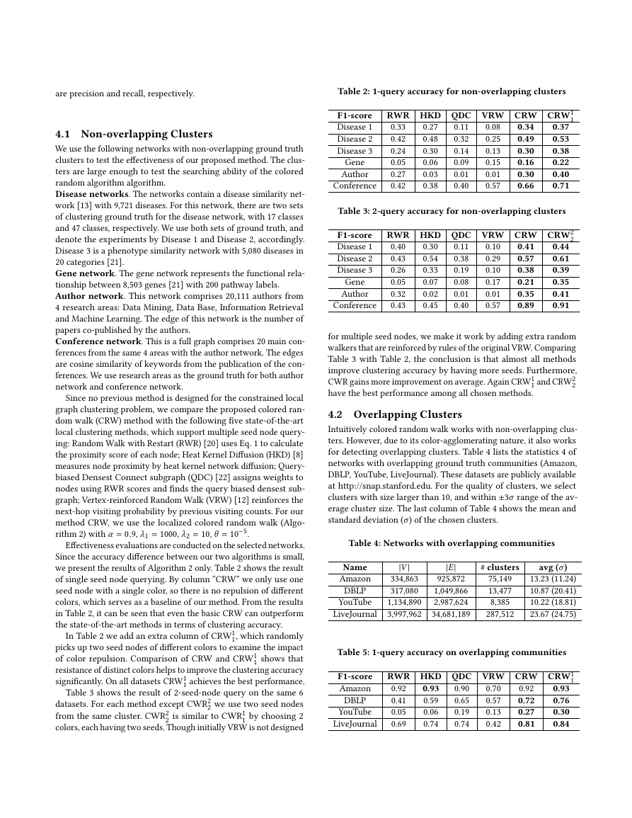
nity. However, when seed nodes are from distinct communities, the
other methods cannot use this relationship, so their performances
are very low (Fig. 4). On the contrary, our method takes advantage
of this cannot-link information, resulting in the increased accuracy
with more communities (colors).
We also evaluate the efficiency of the selected methods on datasets
provided in Table 4, since networks are relatively large. To be fair,
the running time is measured on single color and single node on
every method. Fig. 5 shows that CRW is one of the fastest methods
of all, comparable to the HKD method, and is generally 100 times
faster than the other approaches. Generally, CRW takes no more
than 200 milliseconds in finding a target local cluster. For the scala-
bility of colors and seed nodes, the running time of CRW does not
increase with number of seed nodes, and is proportional with the
number of colors.
4.3 Impact of Color Attraction and Repulsion
To analyze the sensitivity of the main parameters of our method
(λ1, λ2, θ), we generate synthetic networks by the standard LFR
benchmark [10].
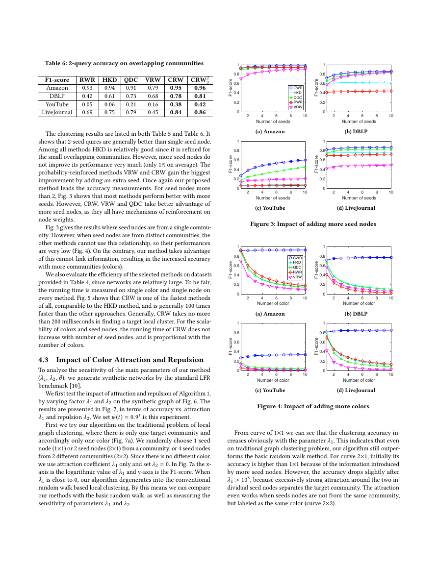
We first test the impact of attraction and repulsion of Algorithm 1,
by varying factor λ1 and λ2 on the synthetic graph of Fig. 6. The
results are presented in Fig. 7, in terms of accuracy vs. attraction
λ1 and repulsion λ2. We set ψ (t ) = 0.9t is this experiment.
First we try our algorithm on the traditional problem of local
graph clustering, where there is only one target community and
accordingly only one color (Fig. 7a). We randomly choose 1 seed
node (1×1) or 2 seed nodes (2×1) from a community, or 4 seed nodes
from 2 different communities (2×2). Since there is no different color,
we use attraction coefficient λ1 only and set λ2 = 0. In Fig. 7a the x-
axis is the logarithmic value of λ1 and y-axis is the F1-score. When
λ1 is close to 0, our algorithm degenerates into the conventional
random walk based local clustering. By this means we can compare
our methods with the basic random walk, as well as measuring the
sensitivity of parameters λ1 and λ2.
(a) Amazon
(b) DBLP
(c) YouTube
(d) LiveJournal
Figure 3: Impact of adding more seed nodes
(a) Amazon
(b) DBLP
(c) YouTube
(d) LiveJournal
Figure 4: Impact of adding more colors
From curve of 1×1 we can see that the clustering accuracy in-
creases obviously with the parameter λ1. This indicates that even
on traditional graph clustering problem, our algorithm still outper-
forms the basic random walk method. For curve 2×1, initially its
accuracy is higher than 1×1 because of the information introduced
by more seed nodes. However, the accuracy drops slightly after
λ1 > 103, because excessively strong attraction around the two in-
dividual seed nodes separates the target community. The attraction
even works when seeds nodes are not from the same community,
but labeled as the same color (curve 2×2).
246810Number of seeds00.20.40.60.81F1-scoreCWRHKDQDCRWRVRW246810Number of seeds00.20.40.60.81F1-score246810Number of seeds00.20.40.60.81F1-score246810Number of seeds00.20.40.60.81F1-score246810Number of color00.20.40.60.81F1-scoreCWRHKDQDCRWRVRW246810Number of color00.20.40.60.81F1-score246810Number of color00.20.40.60.81F1-score246810Number of color00.20.40.60.81F1-score�
Figure 5: Running time comparison
(a) Attraction only
(b) Repulsion only
(c) 1×2 attraction and repulsion (d) 2×2 attraction and repulsion
Community 3
Figure 7: Impact of color attraction and repulsion. λ1 is the
attraction coefficient and λ2 is the repulsion coefficient.
Community 2
Community 1
Figure 6: A 100-node graph generated by the LFR bench-
mark. The red, blue, green nodes are from 3 distinct ground-
truth communities.
Similar results are observed by using repulsion force only and set
λ1 = 0. In experiments shown in Fig. 7b, we select 1 or 2 nodes from
two adjacent communities and label them with different colors. The
figures illustrate that the repulsion enhances clustering accuracy, as
walkers from the two different communities are divided by distinct
colors. However, overdose of repulsion (λ2 > 10) drives walkers
from the border of communities and decreases the accuracy.
Finally, we combine both attraction and repulsion forces together
(shown in Fig. 7c and 7d). The best accuracy results come with
λ1 = 104 and λ2 = 102, and the performance are maintained when
these two parameters keep on increasing. The favorable λ1 and λ2
are large because of the stabilizer “1” in color reinforcement (Eq. 3),
which requires large λ1 and λ2 to change the behavior of random
walkers.
4.4 Evaluation of Speedup Strategy
We generate a network with 1 million nodes and 15 million edges
by LFR benchmark to test the impact of threshold θ on Algorithm 2.
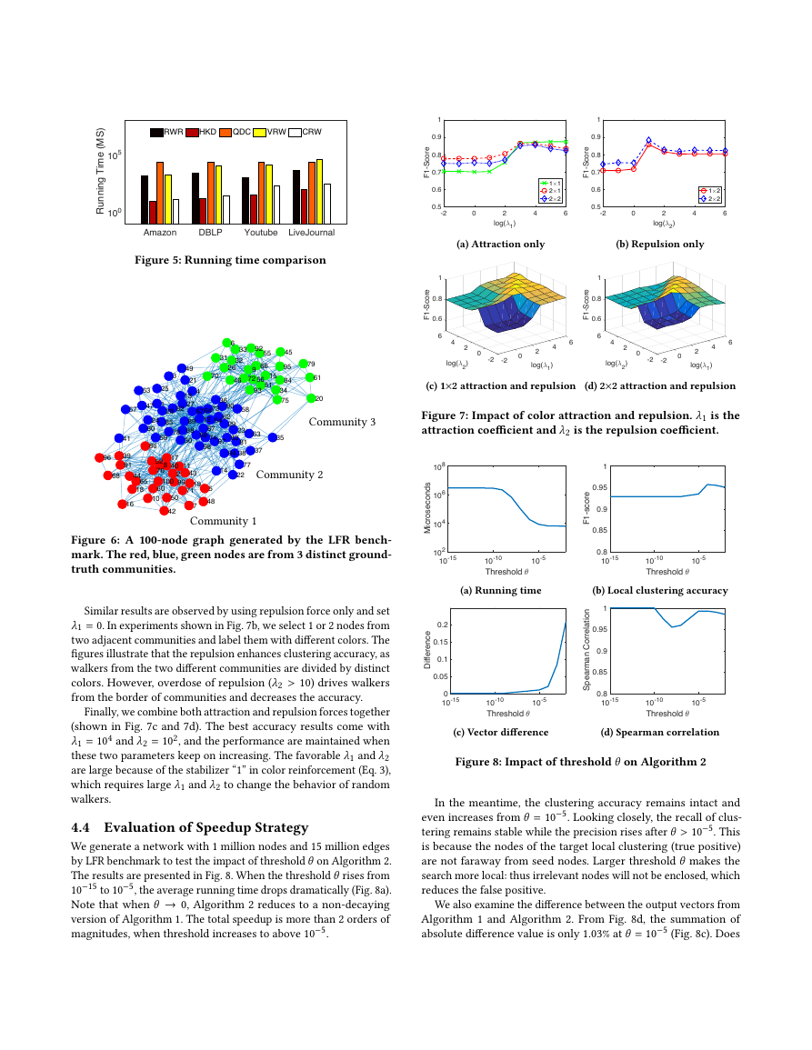
The results are presented in Fig. 8. When the threshold θ rises from
10−15 to 10−5, the average running time drops dramatically (Fig. 8a).
Note that when θ → 0, Algorithm 2 reduces to a non-decaying
version of Algorithm 1. The total speedup is more than 2 orders of
magnitudes, when threshold increases to above 10−5.
(a) Running time
(b) Local clustering accuracy
(c) Vector difference
(d) Spearman correlation
Figure 8: Impact of threshold θ on Algorithm 2
In the meantime, the clustering accuracy remains intact and
even increases from θ = 10−5. Looking closely, the recall of clus-
tering remains stable while the precision rises after θ > 10−5. This
is because the nodes of the target local clustering (true positive)
are not faraway from seed nodes. Larger threshold θ makes the
search more local: thus irrelevant nodes will not be enclosed, which
reduces the false positive.
We also examine the difference between the output vectors from
Algorithm 1 and Algorithm 2. From Fig. 8d, the summation of
absolute difference value is only 1.03% at θ = 10−5 (Fig. 8c). Does
AmazonDBLPYoutubeLiveJournal100105Running Time (MS)RWRHKDQDCVRWCRW-5-4-3-2-1012345-5-4-3-2-1012345 1 2 3 4 5 6 7 8 9 10 11 12 13 14 15 16 17 18 19 20 21 22 23 24 25 26 27 28 29 30 31 32 33 34 35 36 37 38 39 40 41 42 43 44 45 46 47 48 49 50 51 52 53 54 55 56 57 58 59 60 61 62 63 64 65 66 67 68 69 70 71 72 73 74 75 76 77 78 79 80 81 82 83 84 85 86 87 88 89 90 91 92 93 94 95 96 97 98 99 100-20246log(61)0.50.60.70.80.91F1-Score1#12#12#2-20246log(62)0.50.60.70.80.91F1-Score1#22#260.646F1-Score0.84log(62)2log(61)1200-2-260.646F1-Score0.84log(62)2log(61)1200-2-210-1510-1010-5Threshold 3102104106108Microseconds10-1510-1010-5Threshold 30.80.850.90.951F1-score10-1510-1010-5Threshold 300.050.10.150.2Difference10-1510-1010-5Threshold 30.80.850.90.951Spearman Correlation�


 2023年江西萍乡中考道德与法治真题及答案.doc
 2012年重庆南川中考生物真题及答案.doc
 2013年江西师范大学地理学综合及文艺理论基础考研真题.doc
 2020年四川甘孜小升初语文真题及答案I卷.doc
 2020年注册岩土工程师专业基础考试真题及答案.doc
 2023-2024学年福建省厦门市九年级上学期数学月考试题及答案.doc
 2021-2022学年辽宁省沈阳市大东区九年级上学期语文期末试题及答案.doc
 2022-2023学年北京东城区初三第一学期物理期末试卷及答案.doc
 2018上半年江西教师资格初中地理学科知识与教学能力真题及答案.doc
 2012年河北国家公务员申论考试真题及答案-省级.doc
 2020-2021学年江苏省扬州市江都区邵樊片九年级上学期数学第一次质量检测试题及答案.doc
 2022下半年黑龙江教师资格证中学综合素质真题及答案.doc