Fast and Accurate Entity Recognition with Iterated Dilated Convolutions
Emma Strubell
Patrick Verga
David Belanger
College of Information and Computer Sciences
{strubell, pat, belanger, mccallum}@cs.umass.edu
University of Massachusetts Amherst
Andrew McCallum
7
1
0
2
l
u
J
2
2
]
L
C
.
s
c
[
3
v
8
9
0
2
0
.
2
0
7
1
:
v
i
X
r
a
Abstract
Today when many practitioners run basic
NLP on the entire web and large-volume
traffic, faster methods are paramount to
saving time and energy costs. Recent
advances in GPU hardware have led to
the emergence of bi-directional LSTMs
as a standard method for obtaining per-
token vector representations serving as in-
put to labeling tasks such as NER (often
followed by prediction in a linear-chain
CRF). Though expressive and accurate,
these models fail to fully exploit GPU par-
allelism, limiting their computational ef-
ficiency. This paper proposes a faster al-
ternative to Bi-LSTMs for NER: Iterated
Dilated Convolutional Neural Networks
(ID-CNNs), which have better capacity
than traditional CNNs for large context
and structured prediction. Unlike LSTMs
whose sequential processing on sentences
of length N requires O(N ) time even in
the face of parallelism, ID-CNNs permit
fixed-depth convolutions to run in paral-
lel across entire documents. We describe
a distinct combination of network struc-
ture, parameter sharing and training pro-
cedures that enable dramatic 14-20x test-
time speedups while retaining accuracy
comparable to the Bi-LSTM-CRF. More-
over, ID-CNNs trained to aggregate con-
text from the entire document are even
more accurate while maintaining 8x faster
test time speeds.
Introduction
1
In order to democratize large-scale NLP and in-
formation extraction while minimizing our en-
vironmental footprint, we require fast, resource-
efficient methods for sequence tagging tasks such
as part-of-speech tagging and named entity recog-
nition (NER). Speed is not sufficient of course:
they must also be expressive enough to tolerate the
tremendous lexical variation in input data.
The massively parallel computation facilitated
by GPU hardware has led to a surge of success-
ful neural network architectures for sequence la-
beling (Ling et al., 2015; Ma and Hovy, 2016;
Chiu and Nichols, 2016; Lample et al., 2016).
While these models are expressive and accurate,
they fail to fully exploit the parallelism opportu-
nities of a GPU, and thus their speed is limited.
Specifically, they employ either recurrent neural
networks (RNNs) for feature extraction, or Viterbi
inference in a structured output model, both of
which require sequential computation across the
length of the input.
Instead, parallelized runtime independent of the
length of the sequence saves time and energy
costs, maximizing GPU resource usage and min-
imizing the amount of time it takes to train and
evaluate models. Convolutional neural networks
(CNNs) provide exactly this property (Kim, 2014;
Kalchbrenner et al., 2014). Rather than compos-
ing representations incrementally over each token
in a sequence, they apply filters in parallel across
the entire sequence at once. Their computational
cost grows with the number of layers, but not the
input size, up to the memory and threading limita-
tions of the hardware. This provides, for example,
audio generation models that can be trained in par-
allel (van den Oord et al., 2016).
Despite the clear computational advantages of
CNNs, RNNs have become the standard method
for composing deep representations of text. This is
because a token encoded by a bidirectional RNN
will incorporate evidence from the entire input se-
quence, but the CNN’s representation is limited by
�
the effective input width1 of the network: the size
of the input context which is observed, directly
or indirectly, by the representation of a token at
a given layer in the network. Specifically, in a
network composed of a series of stacked convo-
lutional layers of convolution width w, the num-
ber r of context tokens incorporated into a to-
ken’s representation at a given layer l, is given by
r = l(w − 1) + 1. The number of layers required
to incorporate the entire input context grows lin-
early with the length of the sequence. To avoid this
scaling, one could pool representations across the
sequence, but this is not appropriate for sequence
labeling, since it reduces the output resolution of
the representation.
In response, this paper presents an application
of dilated convolutions (Yu and Koltun, 2016) for
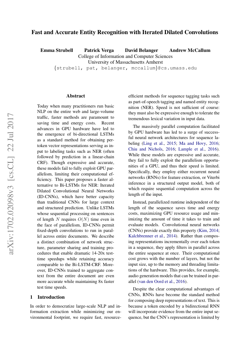
sequence labeling (Figure 1). For dilated convo-
lutions, the effective input width can grow expo-
nentially with the depth, with no loss in resolu-
tion at each layer and with a modest number of
parameters to estimate. Like typical CNN layers,
dilated convolutions operate on a sliding window
of context over the sequence, but unlike conven-
tional convolutions, the context need not be con-
secutive; the dilated window skips over every dila-
tion width d inputs. By stacking layers of dilated
convolutions of exponentially increasing dilation
width, we can expand the size of the effective input
width to cover the entire length of most sequences
using only a few layers: The size of the effective
input width for a token at layer l is now given by
2l+1−1. More concretely, just four stacked dilated
convolutions of width 3 produces token represen-
tations with a n effective input width of 31 tokens
– longer than the average sentence length (23) in
the Penn TreeBank.
Our overall iterated dilated CNN architecture
(ID-CNN) repeatedly applies the same block of di-
lated convolutions to token-wise representations.
This parameter sharing prevents overfitting and
also provides opportunities to inject supervision
on intermediate activations of the network. Simi-
lar to models that use logits produced by an RNN,
the ID-CNN provides two methods for perform-
ing prediction: we can predict each token’s label
independently, or by running Viterbi inference in
a chain structured graphical model.
In experiments on CoNLL 2003 and OntoNotes
Figure 1: A dilated CNN block with maximum
dilation width 4 and filter width 3. Neurons con-
tributing to a single highlighted neuron in the last
layer are also highlighted.
5.0 English NER, we demonstrate significant
speed gains of our ID-CNNs over various recur-
rent models, while maintaining similar F1 perfor-
mance. When performing prediction using inde-
pendent classification, the ID-CNN consistently
outperforms a bidirectional LSTM (Bi-LSTM),
and performs on par with inference in a CRF
with logits from a Bi-LSTM (Bi-LSTM-CRF). As
an extractor of per-token logits for a CRF, our
model out-performs the Bi-LSTM-CRF. We also
apply ID-CNNs to entire documents, where inde-
pendent token classification is as accurate as the
Bi-LSTM-CRF while decoding almost 8× faster.
The clear accuracy gains resulting from incorpo-
rating broader context suggest that these mod-
els could similarly benefit many other context-
sensitive NLP tasks which have until now been
limited by the computational complexity of exist-
ing context-rich models.2
2 Background
2.1 Conditional Probability Models for
Tagging
Let x = [x1, . . . , xT ] be our input text and y =
[y1, . . . , yT ] be per-token output tags. Let D be
the domain size of each yi. We predict the most
likely y, given a conditional model P (y|x).
This paper considers two factorizations of the
conditional distribution. First, we have
T
P (y|x) =
P (yt|F (x)),
(1)
t=1
where the tags are conditionally independent given
some features for x. Given these features, O(D)
prediction is simple and parallelizable across the
1What we call effective input width here is known as the
receptive field in the vision literature, drawing an analogy to
the visual receptive field of a neuron in the retina.
2Our
implementation in TensorFlow (Abadi et al.,
2015) is available at: https://github.com/iesl/
dilated-cnn-ner
�
length of the sequence. However, feature extrac-
tion may not necessarily be parallelizable. For
example, RNN-based features require iterative
passes along the length of x.
We also consider a linear-chain CRF model that
couples all of y together:
P (y|x) =
1
Zx
ψt(yt|F (x))ψp(yt, yt−1),
(2)
T
t=1
where ψt is a local factor, ψp is a pairwise factor
that scores consecutive tags, and Zx is the parti-
tion function (Lafferty et al., 2001). To avoid over-
fitting, ψp does not depend on the timestep t or
the input x in our experiments. Prediction in this
model requires global search using the O(D2T )
Viterbi algorithm.
CRF prediction explicitly reasons about inter-
actions among neighboring output tags, whereas
prediction in the first model compiles this reason-
ing into the feature extraction step (Liang et al.,
2008). The suitability of such compilation de-
pends on the properties and quantity of the data.
While CRF prediction requires non-trivial search
in output space, it can guarantee that certain output
constraints, such as for IOB tagging (Ramshaw
and Marcus, 1999), will always be satisfied.
It
may also have better sample complexity, as it im-
poses more prior knowledge about the structure
of the interactions among the tags (London et al.,
2016). However, it has worse computational com-
plexity than independent prediction.
3 Dilated Convolutions
CNNs in NLP are typically one-dimensional, ap-
plied to a sequence of vectors representing tokens
rather than to a two-dimensional grid of vectors
representing pixels. In this setting, a convolutional
neural network layer is equivalent to applying an
affine transformation, Wc to a sliding window of
width r tokens on either side of each token in the
sequence. Here, and throughout the paper, we do
not explicitly write the bias terms in affine trans-
formations. The convolutional operator applied to
each token xt with output ct is defined as:
ct = Wc
xt±k,
(3)
where ⊕ is vector concatenation.
k=0
Dilated convolutions perform the same opera-
tion, except rather than transforming adjacent in-
r
r
puts, the convolution is defined over a wider ef-
fective input width by skipping over δ inputs at a
time, where δ is the dilation width. We define the
dilated convolution operator:
ct = Wc
xt±kδ.
(4)
k=0
A dilated convolution of width 1 is equivalent to
a simple convolution. Using the same number of
parameters as a simple convolution with the same
radius (i.e. Wc has the same dimensionality), the
δ > 1 dilated convolution incorporates broader
context into the representation of a token than a
simple convolution.
3.1 Multi-Scale Context Aggregation
We can leverage the ability of dilated convolutions
to incorporate global context without losing im-
portant local information by stacking dilated con-
volutions of increasing width. First described for
pixel classification in computer vision, Yu and
Koltun (2016) achieve state-of-the-art results on
image segmentation benchmarks by stacking di-
lated convolutions with exponentially increasing
rates of dilation, a technique they refer to as multi-
scale context aggregation. By feeding the out-
puts of each dilated convolution as the input to the
next, increasingly non-local information is incor-
porated into each pixel’s representation. Perform-
ing a dilation-1 convolution in the first layer en-
sures that no pixels within the effective input width
of any pixel are excluded. By doubling the dila-
tion width at each layer, the size of the effective
input width grows exponentially while the number
of parameters grows only linearly with the number
of layers, so a pixel representation quickly incor-
porates rich global evidence from the entire im-
age.
4
Iterated Dilated CNNs
Stacked dilated CNNs can easily incorporate
global information from a whole sentence or docu-
ment. For example, with a radius of 1 and 4 layers
of dilated convolutions, the effective input width
of each token is width 31, which exceeds the av-
erage sentence length (23) in the Penn TreeBank
corpus. With a radius of size 2 and 8 layers of
dilated convolutions, the effective input width ex-
ceeds 1,000 tokens, long enough to encode a full
newswire document.
�
Unfortunately, simply increasing the depth of
stacked dilated CNNs causes considerable over-
fitting in our experiments. In response, we present
Iterated Dilated CNNs (ID-CNNs), which instead
apply the same small stack of dilated convolutions
multiple times, each iterate taking as input the re-
sult of the last application. Repeatedly employing
the same parameters in a recurrent fashion pro-
vides both broad effective input width and desir-
able generalization capabilities. We also obtain
significant accuracy gains with a training objec-
tive that strives for accurate labeling after each it-
erate, allowing follow-on iterations to observe and
resolve dependency violations.
4.1 Model Architecture
The network takes as input a sequence of T vec-
tors xt, and outputs a sequence of per-class scores
ht, which serve either as the local conditional dis-
tributions of Eqn. (1) or the local factors ψt of
Eqn. (2).
We denote the jth dilated convolutional layer of
. The first layer in the net-
that trans-
dilation width δ as D(j)
δ
work is a dilation-1 convolution D(0)
1
forms the input to a representation it:
it = D(0)
1 xt
(5)
Next, Lc layers of dilated convolutions of expo-
nentially increasing dilation width are applied to
it, folding in increasingly broader context into the
embedded representation of xt at each layer. Let
r() denote the ReLU activation function (Glorot
et al., 2011). Beginning with ct
(0) = it we define
the stack of layers with the following recurrence:
and add a final dilation-1 layer to the stack:
ct
(j) = r
D(j−1)
2Lc−1ct
ct
(Lc+1) = r
D(Lc)
1
ct
(j−1)
(Lc)
(6)
(7)
We refer to this stack of dilated convolutions as a
block B(·), which has output resolution equal to
its input resolution. To incorporate even broader
context without over-fitting, we avoid making B
deeper, and instead iteratively apply B Lb times,
introducing no extra parameters. Starting with
bt
(1) = B (it):
(k−1)
bt
(k) = B
bt
We apply a simple affine transformation Wo to this
final representation to obtain per-class scores for
each token xt:
ht
(Lb) = Wobt
(Lb)
(9)
4.2 Training
Our main focus is to apply the ID-CNN an en-
coder to produce per-token logits for the first con-
ditional model described in Sec. 2.1, where tags
are conditionally independent given deep features,
since this will enable prediction that is paralleliz-
able across the length of the input sequence. Here,
maximum likelihood training is straightforward
because the likelihood decouples into the sum of
the likelihoods of independent logistic regression
problems for every tag, with natural parameters
given by Eqn. (9):
log P (yt | ht
(Lb))
(10)
T
t=1
1
T
We can also use the ID-CNN as logits for
the CRF model (Eqn. (2)), where the partition
function and its gradient are computed using the
forward-backward algorithm.
We next present an alternative training method
that helps bridge the gap between these two tech-
niques. Sec. 2.1 identifies that the CRF has prefer-
able sample complexity and accuracy since pre-
diction directly reasons in the space of structured
outputs. In response, we compile some of this rea-
soning in output space into ID-CNN feature ex-
traction. Instead of explicit reasoning over output
labels during inference, we train the network such
that each block is predictive of output labels. Sub-
sequent blocks learn to correct dependency viola-
tions of their predecessors, refining the final se-
quence prediction.
To do so, we first define predictions of the
model after each of the Lb applications of the
(k) be the result of applying the ma-
block. Let ht
(k), the output of block k.
trix Wo from (9) to bt
We minimize the average of the losses for each
application of the block:
T
Lb
1
T
k=1
t=1
1
Lb
log P (yt | ht
(k)).
(11)
By rewarding accurate predictions after each
application of the block, we learn a model where
later blocks are used to refine initial predictions.
(8)
�
The loss also helps reduce the vanishing gradi-
ent problem (Hochreiter, 1998) for deep architec-
tures. Such an approach has been applied in a va-
riety of contexts for training very deep networks
in computer vision (Romero et al., 2014; Szegedy
et al., 2015; Lee et al., 2015; G¨ulc¸ehre and Bengio,
2016), but not to our knowledge in NLP.
We apply dropout (Srivastava et al., 2014) to the
(b) to
raw inputs xt and to each block’s output bt
help prevent overfitting. The version of dropout
typically used in practice has the undesirable prop-
erty that the randomized predictor used at train
time differs from the fixed one used at test time.
Ma et al. (2017) present dropout with expectation-
linear regularization, which explicitly regularizes
these two predictors to behave similarly. All of our
best reported results include such regularization.
This is the first investigation of the technique’s ef-
fectiveness for NLP, including for RNNs. We en-
courage its further application.
5 Related work
The state-of-the art models for sequence labeling
include an inference step that searches the space
of possible output sequences of a chain-structured
graphical model, or approximates this search with
a beam (Collobert et al., 2011; Weiss et al., 2015;
Lample et al., 2016; Ma and Hovy, 2016; Chiu and
Nichols, 2016). These outperform similar systems
that use the same features, but independent local
predictions. On the other hand, the greedy sequen-
tial prediction (Daum´e III et al., 2009) approach
of Ratinov and Roth (2009), which employs lex-
icalized features, gazetteers, and word clusters,
outperforms CRFs with similar features.
LSTMs (Hochreiter and Schmidhuber, 1997)
were used for NER as early as the CoNLL
shared task in 2003 (Hammerton, 2003; Tjong
Kim Sang and De Meulder, 2003). More re-
cently, a wide variety of neural network architec-
tures for NER have been proposed. Collobert et al.
(2011) employ a one-layer CNN with pre-trained
word embeddings, capitalization and lexicon fea-
tures, and CRF-based prediction. Huang et al.
(2015) achieved state-of-the-art accuracy on part-
of-speech, chunking and NER using a Bi-LSTM-
CRF. Lample et al. (2016) proposed two mod-
els which incorporated Bi-LSTM-composed char-
acter embeddings alongside words: a Bi-LSTM-
CRF, and a greedy stack LSTM which uses a
simple shift-reduce grammar to compose words
into labeled entities. Their Bi-LSTM-CRF ob-
tained the state-of-the-art on four languages with-
out word shape or lexicon features. Ma and Hovy
(2016) use CNNs rather than LSTMs to compose
characters in a Bi-LSTM-CRF, achieving state-of-
the-art performance on part-of-speech tagging and
CoNLL NER without lexicons. Chiu and Nichols
(2016) evaluate a similar network but propose a
novel method for encoding lexicon matches, pre-
senting results on CoNLL and OntoNotes NER.
Yang et al. (2016) use GRU-CRFs with GRU-
composed character embeddings of words to train
a single network on many tasks and languages.
In general, distributed representations for text
can provide useful generalization capabilities for
NER systems, since they can leverage unsuper-
vised pre-training of distributed word representa-
tions (Turian et al., 2010; Collobert et al., 2011;
Passos et al., 2014). Though our models would
also likely benefit from additional features such as
character representations and lexicons, we focus
on simpler models which use word-embeddings
alone, leaving more elaborate input representa-
tions to future work.
In these NER approaches, CNNs were used for
low-level feature extraction that feeds into alter-
native architectures. Overall, end-to-end CNNs
have mainly been used in NLP for sentence classi-
fication, where the output representation is lower
resolution than that of the input Kim (2014);
Kalchbrenner et al. (2014); Zhang et al. (2015);
Toutanova et al. (2015). Lei et al. (2015) present
a CNN variant where convolutions adaptively skip
neighboring words. While the flexibility of this
model is powerful, its adaptive behavior is not
well-suited to GPU acceleration.
Our work draws on the use of dilated convolu-
tions for image segmentation in the computer vi-
sion community (Yu and Koltun, 2016; Chen et al.,
2015). Similar to our block, Yu and Koltun (2016)
employ a context-module of stacked dilated convo-
lutions of exponentially increasing dilation width.
Dilated convolutions were recently applied to the
task of speech generation (van den Oord et al.,
2016), and concurrent with this work, Kalchbren-
ner et al. (2016) posted a pre-print describing the
similar ByteNet network for machine translation
that uses dilated convolutions in the encoder and
decoder components. Our basic model architec-
ture is similar to that of the ByteNet encoder, ex-
cept that the inputs to our model are tokens and
�
not bytes. Additionally, we present a novel loss
and parameter sharing scheme to facilitate training
models on much smaller datasets than those used
by Kalchbrenner et al. (2016). We are the first to
use dilated convolutions for sequence labeling.
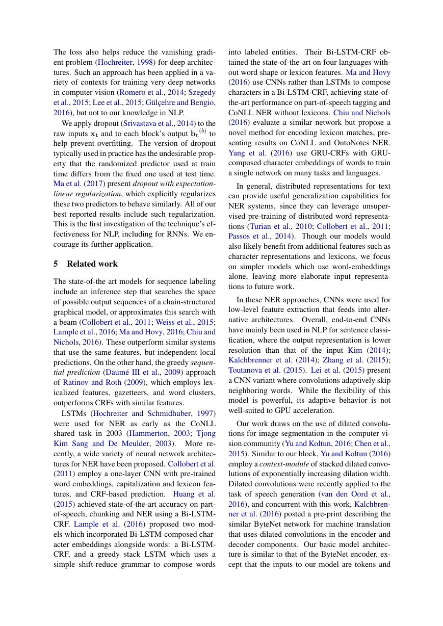
The broad effective input width of the ID-CNN
helps aggregate document-level context. Ratinov
and Roth (2009) incorporate document context in
their greedy model by adding features based on
tagged entities within a large, fixed window of to-
kens. Prior work has also posed a structured model
that couples predictions across the whole docu-
ment (Bunescu and Mooney, 2004; Sutton and
McCallum, 2004; Finkel et al., 2005).
6 Experimental Results
We describe experiments on two benchmark En-
glish named entity recognition datasets. On
CoNLL-2003 English NER, our ID-CNN per-
forms on par with a Bi-LSTM not only when used
to produce per-token logits for structured infer-
ence, but the ID-CNN with greedy decoding also
performs on-par with the Bi-LSTM-CRF while
running at more than 14 times the speed. We also
observe a performance boost in almost all models
when broadening the context to incorporate entire
documents, achieving an average F1 of 90.65 on
CoNLL-2003, out-performing the sentence-level
model while still decoding at nearly 8 times the
speed of the Bi-LSTM-CRF.
6.1 Data and Evaluation
We evaluate using labeled data from the CoNLL-
2003 shared task (Tjong Kim Sang and De Meul-
der, 2003) and OntoNotes 5.0 (Hovy et al., 2006;
Pradhan et al., 2006). Following previous work,
we use the same OntoNotes data split used for
co-reference resolution in the CoNLL-2012 shared
task (Pradhan et al., 2012). For both datasets, we
convert the IOB boundary encoding to BILOU as
previous work found this encoding to result in im-
proved performance (Ratinov and Roth, 2009). As
in previous work we evaluate the performance of
our models using segment-level micro-averaged
F1 score. Hyperparameters that resulted in the
best performance on the validation set were se-
lected via grid search. A more detailed descrip-
tion of the data, evaluation, optimization and data
pre-processing can be found in the Appendix.
6.2 Baselines
We compare our ID-CNN against strong LSTM
and CNN baselines: a Bi-LSTM with local de-
coding, and one with CRF decoding (Bi-LSTM-
CRF). We also compare against a non-dilated
CNN architecture with the same number of con-
volutional layers as our dilated network (4-layer
CNN) and one with enough layers to incorporate
an effective input width of the same size as that
of the dilated network (5-layer CNN) to demon-
strate that the dilated convolutions more effec-
tively aggregate contextual information than sim-
ple convolutions (i.e. using fewer parameters). We
also compare our document-level ID-CNNs to a
baseline which does not share parameters between
blocks (noshare) and one that computes loss only
at the last block, rather than after every iterated
block of dilated convolutions (1-loss).
We do not compare with deeper or more elab-
orate CNN architectures for a number of reasons:
1) Fast train and test performance are highly desir-
able for NLP practitioners, and deeper models re-
quire more computation time 2) more complicated
models tend to over-fit on this relatively small
dataset and 3) most accurate deep CNN architec-
tures repeatedly up-sample and down-sample the
inputs. We do not compare to stacked LSTMs
for similar reasons — a single LSTM is already
slower than a 4-layer CNN. Since our task is se-
quence labeling, we desire a model that maintains
the token-level resolution of the input, making di-
lated convolutions an elegant solution.
6.3 CoNLL-2003 English NER
6.3.1 Sentence-level prediction
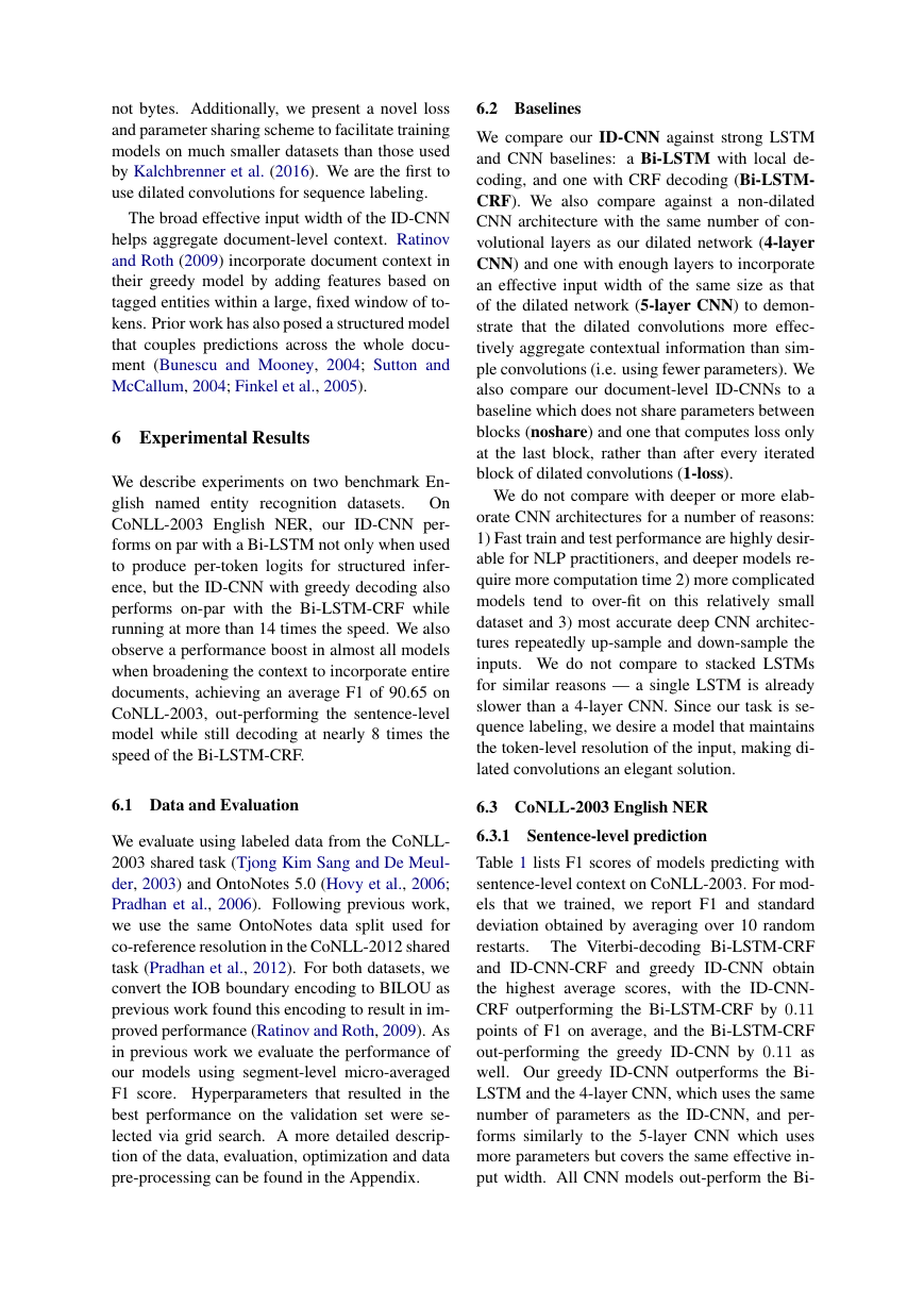
Table 1 lists F1 scores of models predicting with
sentence-level context on CoNLL-2003. For mod-
els that we trained, we report F1 and standard
deviation obtained by averaging over 10 random
restarts.
The Viterbi-decoding Bi-LSTM-CRF
and ID-CNN-CRF and greedy ID-CNN obtain
the highest average scores, with the ID-CNN-
CRF outperforming the Bi-LSTM-CRF by 0.11
points of F1 on average, and the Bi-LSTM-CRF
out-performing the greedy ID-CNN by 0.11 as
well. Our greedy ID-CNN outperforms the Bi-
LSTM and the 4-layer CNN, which uses the same
number of parameters as the ID-CNN, and per-
forms similarly to the 5-layer CNN which uses
more parameters but covers the same effective in-
put width. All CNN models out-perform the Bi-
�
Model
Ratinov and Roth (2009)
Collobert et al. (2011)
Lample et al. (2016)
Bi-LSTM
4-layer CNN
5-layer CNN
ID-CNN
Collobert et al. (2011)
Passos et al. (2014)
Lample et al. (2016)
Bi-LSTM-CRF (re-impl)
ID-CNN-CRF
F1
86.82
86.96
90.33
89.34 ± 0.28
89.97 ± 0.20
90.23 ± 0.16
90.32 ± 0.26
88.67
90.05
90.20
90.43 ± 0.12
90.54 ± 0.18
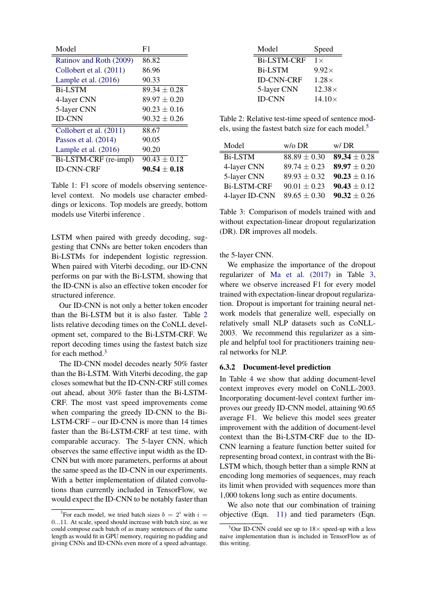
Table 1: F1 score of models observing sentence-
level context. No models use character embed-
dings or lexicons. Top models are greedy, bottom
models use Viterbi inference .
LSTM when paired with greedy decoding, sug-
gesting that CNNs are better token encoders than
Bi-LSTMs for independent
logistic regression.
When paired with Viterbi decoding, our ID-CNN
performs on par with the Bi-LSTM, showing that
the ID-CNN is also an effective token encoder for
structured inference.
Our ID-CNN is not only a better token encoder
than the Bi-LSTM but it is also faster. Table 2
lists relative decoding times on the CoNLL devel-
opment set, compared to the Bi-LSTM-CRF. We
report decoding times using the fastest batch size
for each method.3
The ID-CNN model decodes nearly 50% faster
than the Bi-LSTM. With Viterbi decoding, the gap
closes somewhat but the ID-CNN-CRF still comes
out ahead, about 30% faster than the Bi-LSTM-
CRF. The most vast speed improvements come
when comparing the greedy ID-CNN to the Bi-
LSTM-CRF – our ID-CNN is more than 14 times
faster than the Bi-LSTM-CRF at test time, with
comparable accuracy. The 5-layer CNN, which
observes the same effective input width as the ID-
CNN but with more parameters, performs at about
the same speed as the ID-CNN in our experiments.
With a better implementation of dilated convolu-
tions than currently included in TensorFlow, we
would expect the ID-CNN to be notably faster than
3For each model, we tried batch sizes b = 2i with i =
0...11. At scale, speed should increase with batch size, as we
could compose each batch of as many sentences of the same
length as would fit in GPU memory, requiring no padding and
giving CNNs and ID-CNNs even more of a speed advantage.
Speed
Model
Bi-LSTM-CRF 1×
Bi-LSTM
ID-CNN-CRF
5-layer CNN
ID-CNN
9.92×
1.28×
12.38×
14.10×
Table 2: Relative test-time speed of sentence mod-
els, using the fastest batch size for each model.5
w/ DR
Model
w/o DR
89.34 ± 0.28
88.89 ± 0.30
Bi-LSTM
89.97 ± 0.20
89.74 ± 0.23
4-layer CNN
90.23 ± 0.16
89.93 ± 0.32
5-layer CNN
90.43 ± 0.12
90.01 ± 0.23
Bi-LSTM-CRF
90.32 ± 0.26
4-layer ID-CNN 89.65 ± 0.30
Table 3: Comparison of models trained with and
without expectation-linear dropout regularization
(DR). DR improves all models.
the 5-layer CNN.
(2017)
We emphasize the importance of the dropout
regularizer of Ma et al.
in Table 3,
where we observe increased F1 for every model
trained with expectation-linear dropout regulariza-
tion. Dropout is important for training neural net-
work models that generalize well, especially on
relatively small NLP datasets such as CoNLL-
2003. We recommend this regularizer as a sim-
ple and helpful tool for practitioners training neu-
ral networks for NLP.
6.3.2 Document-level prediction
In Table 4 we show that adding document-level
context improves every model on CoNLL-2003.
Incorporating document-level context further im-
proves our greedy ID-CNN model, attaining 90.65
average F1. We believe this model sees greater
improvement with the addition of document-level
context than the Bi-LSTM-CRF due to the ID-
CNN learning a feature function better suited for
representing broad context, in contrast with the Bi-
LSTM which, though better than a simple RNN at
encoding long memories of sequences, may reach
its limit when provided with sequences more than
1,000 tokens long such as entire documents.
We also note that our combination of training
objective (Eqn. 11) and tied parameters (Eqn.
5Our ID-CNN could see up to 18× speed-up with a less
naive implementation than is included in TensorFlow as of
this writing.
�
Model
4-layer ID-CNN (sent)
Bi-LSTM-CRF (sent)
4-layer CNN × 3
5-layer CNN × 3
Bi-LSTM
Bi-LSTM-CRF
ID-CNN
F1
90.32 ± 0.26
90.43 ± 0.12
90.32 ± 0.32
90.45 ± 0.21
89.09 ± 0.19
90.60 ± 0.19
90.65 ± 0.15
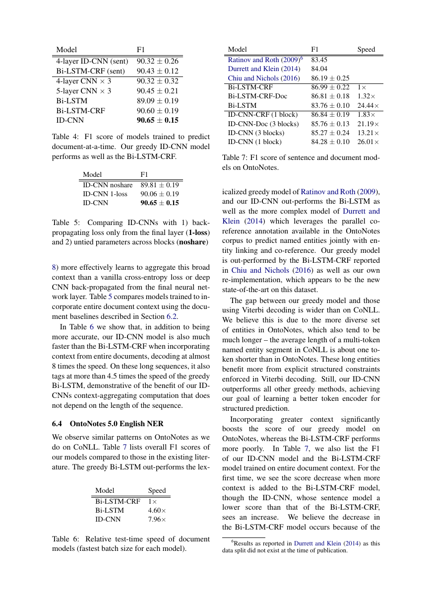
Table 4: F1 score of models trained to predict
document-at-a-time. Our greedy ID-CNN model
performs as well as the Bi-LSTM-CRF.
Model
ID-CNN noshare
ID-CNN 1-loss
ID-CNN
F1
89.81 ± 0.19
90.06 ± 0.19
90.65 ± 0.15
Table 5: Comparing ID-CNNs with 1) back-
propagating loss only from the final layer (1-loss)
and 2) untied parameters across blocks (noshare)
8) more effectively learns to aggregate this broad
context than a vanilla cross-entropy loss or deep
CNN back-propagated from the final neural net-
work layer. Table 5 compares models trained to in-
corporate entire document context using the docu-
ment baselines described in Section 6.2.
In Table 6 we show that, in addition to being
more accurate, our ID-CNN model is also much
faster than the Bi-LSTM-CRF when incorporating
context from entire documents, decoding at almost
8 times the speed. On these long sequences, it also
tags at more than 4.5 times the speed of the greedy
Bi-LSTM, demonstrative of the benefit of our ID-
CNNs context-aggregating computation that does
not depend on the length of the sequence.
6.4 OntoNotes 5.0 English NER
We observe similar patterns on OntoNotes as we
do on CoNLL. Table 7 lists overall F1 scores of
our models compared to those in the existing liter-
ature. The greedy Bi-LSTM out-performs the lex-
Speed
Model
Bi-LSTM-CRF 1×
Bi-LSTM
ID-CNN
4.60×
7.96×
Model
Ratinov and Roth (2009)6
Durrett and Klein (2014)
Chiu and Nichols (2016)
Bi-LSTM-CRF
Bi-LSTM-CRF-Doc
Bi-LSTM
ID-CNN-CRF (1 block)
ID-CNN-Doc (3 blocks)
ID-CNN (3 blocks)
ID-CNN (1 block)
F1
83.45
84.04
86.19 ± 0.25
86.99 ± 0.22
86.81 ± 0.18
83.76 ± 0.10
86.84 ± 0.19
85.76 ± 0.13
85.27 ± 0.24
84.28 ± 0.10
Speed
1×
1.32×
24.44×
1.83×
21.19×
13.21×
26.01×
Table 7: F1 score of sentence and document mod-
els on OntoNotes.
icalized greedy model of Ratinov and Roth (2009),
and our ID-CNN out-performs the Bi-LSTM as
well as the more complex model of Durrett and
Klein (2014) which leverages the parallel co-
reference annotation available in the OntoNotes
corpus to predict named entities jointly with en-
tity linking and co-reference. Our greedy model
is out-performed by the Bi-LSTM-CRF reported
in Chiu and Nichols (2016) as well as our own
re-implementation, which appears to be the new
state-of-the-art on this dataset.
The gap between our greedy model and those
using Viterbi decoding is wider than on CoNLL.
We believe this is due to the more diverse set
of entities in OntoNotes, which also tend to be
much longer – the average length of a multi-token
named entity segment in CoNLL is about one to-
ken shorter than in OntoNotes. These long entities
benefit more from explicit structured constraints
enforced in Viterbi decoding. Still, our ID-CNN
outperforms all other greedy methods, achieving
our goal of learning a better token encoder for
structured prediction.
context
Incorporating greater
significantly
boosts
the score of our greedy model on
OntoNotes, whereas the Bi-LSTM-CRF performs
more poorly.
In Table 7, we also list the F1
of our ID-CNN model and the Bi-LSTM-CRF
model trained on entire document context. For the
first time, we see the score decrease when more
context is added to the Bi-LSTM-CRF model,
though the ID-CNN, whose sentence model a
lower score than that of
the Bi-LSTM-CRF,
sees an increase. We believe the decrease in
the Bi-LSTM-CRF model occurs because of the
Table 6: Relative test-time speed of document
models (fastest batch size for each model).
6Results as reported in Durrett and Klein (2014) as this
data split did not exist at the time of publication.
�


 2023年江西萍乡中考道德与法治真题及答案.doc
 2012年重庆南川中考生物真题及答案.doc
 2013年江西师范大学地理学综合及文艺理论基础考研真题.doc
 2020年四川甘孜小升初语文真题及答案I卷.doc
 2020年注册岩土工程师专业基础考试真题及答案.doc
 2023-2024学年福建省厦门市九年级上学期数学月考试题及答案.doc
 2021-2022学年辽宁省沈阳市大东区九年级上学期语文期末试题及答案.doc
 2022-2023学年北京东城区初三第一学期物理期末试卷及答案.doc
 2018上半年江西教师资格初中地理学科知识与教学能力真题及答案.doc
 2012年河北国家公务员申论考试真题及答案-省级.doc
 2020-2021学年江苏省扬州市江都区邵樊片九年级上学期数学第一次质量检测试题及答案.doc
 2022下半年黑龙江教师资格证中学综合素质真题及答案.doc