Accurate Odometry and Error Modelling for a Mobile Robot, MECSE-1996-6
Accurate Odometry and Error Modelling for a Mobile Robot
Kok Seng CHONG
kok.seng.chong@eng.monash.edu.au
lindsay.kleeman@eng.monash.edu.au
Lindsay KLEEMAN
Intelligent Robotics Research Centre (IRRC)
Department of Electrical and Computer Systems Engineering
Monash University, Clayton Victoria 3168, Australia
http://calvin.eng.monash.edu.au/IRRC/index.html
Abstract
This paper presents a low cost novel odometry design capable of achieving high accuracy dead-
reckoning. It also develops a statistical error model for estimating position and orientation
errors of a mobile robot using odometry. Previous work on propagating odometry error
covariance relies on incrementally updating the covariance matrix in small time steps. The
approach taken here sums the noise theoretically over the entire path length to produce simple
closed form expressions, allowing efficient covariance matrix updating after the completion of
path segments. Closed form error covariance matrix is developed for a general circular arc and
two special cases : (I) straight line and (II) turning about the centre of axle of the robot. Other
paths can be composed of short segments of constant curvature arcs without great loss of
accuracy. The model assumes that wheel distance measurement errors are exclusively random
zero mean white noise. Systematic errors due to wheel radius and wheel base measurement were
first calibrated with UMBmark [BorFen94]. Experimental results show that, despite its low cost,
our system’s performance, with regard to dead-reckoning accuracy, is comparable to some of
the best, award-winning vehicles around. The statistical error model, on the other hand, needs
to be improved in light of new insights.
1 Introduction
One of the major tasks of autonomous robotics navigation is localisation. In a
typical indoor environment with a flat floorplan, localisation becomes a matter of
determining the Cartesian coordinates (x,y) and the orientation θ, collectively known
as the state, of the robot on a two dimensional floorplan. For a typical two wheel
robot, odometry (also known as dead-reckoning) remains to be one of the most
important means of achieving this task. Odometry is the measurement of wheel
rotation as a function of time. If the two wheels of the robot are joined to a common
axle, the position and orientation of the centre of the axle relative to the previous
position and orientation can be determined from odometry measurements on both
wheels. In practice, optical encoders that are mounted onto both drive wheels feed
discretised wheel increment information to the central processor, which in turn
continually updates the robot’s state using geometric equations. However, with time,
odometric localisation accumulates errors in an unbounded fashion due to wheel
slippage, floor roughness and discretised sampling of wheel increments. A lot of
research works have been undergone at both the hardware and theoretical level to
improve the reliability of odometry.
At the hardware level, [BarDur95] determine the position of their robot based
on inertial navigation with gyroscopes and/or accelerometers, but this method has
been proven to be susceptible to drift. The remainder of this paragraph showcases the
dead-reckoning implementations of a few robot vehicles from the University of
Michigan: Cybermotion K2A utilises synchro-drive, which makes it insensitive to
1
�
Accurate Odometry and Error Modelling for a Mobile Robot, MECSE-1996-6
non-systematic errors. CLAPPER, consisted of two TRC LabMates connected by a
compliant linkage, uses two rotary encoders to measure the rotation of the labmates
relative to the compliant linkage, and a linear encoder to measure the relative distance
between their centrepoints, giving it the unique ability to measure and correct non-
systematic dead-reckoning errors during motion. In the attempt to improve the dead-
reckoning performance of a tracked vehicle called Andros, a two-wheeled encoder
trailer is attached to the back of the vehicle, which is able to freely rotate on the
horizontal plane. The rotations of the trailer wheels and the trailer with respect to
Andros are measured with the attached optical encoders. More details about these
robots can be found in [BorFen94]. To the best of the authors’ knowledge, the robot
used in the experiment has a unique, lowest cost mechanical design which differs
from all the existing ones while still achieve comparable accuracy.
Work done at the theoretical level normally involves error quantification via
modelling, so that some kind of mathematical treatment would be possible. For
instance, many robust stochastic based techniques such as the Extended Kalman Filter
(EKF) require that the odometry errors be statistically quantified in the form of an
error covariance matrix, so that it can be combined with the information provided by
the external reference to produce a linear minimum mean square estimate of the
position. Therefore, high level methods also sometimes imply the utilisation of
additional external referencing of position.
Normally, odometry errors can be classified as being systematic or non-
systematic, and it is a common engineering practice to first identify the sources of
systematic errors and have them calibrated prior to using the system. In the work by
Borenstein and Feng [BorFen94], a calibration technique called UMBmark test has
been developed to calibrate out the systematic errors suffered by a typical two wheel
robot. The dominant systematic error sources are identified as being the difference in
wheel diameter and the uncertainty about the effective wheel base. The experiment
designed requires that robot be moved around a square path in both the clockwise
(CW) and counterclockwise (CCW) senses several times. The average Cartesian
offsets, known as the centres of gravity, from the initial positions are assumed to be a
sum (superposition) of the errors contributed by both systematic error sources. The
error model parameters are then solved and incorporated into the software as tuning
factors. In our work, this method has been used to calibrate the robot.
To be able to propagate the error covariance matrix of the robot’s state
following a change of stage is the main focus of this chapter. A commonly used
method [Durra93, Jenki93] is now presented. Supposed the at stage k-1, the state of
the robot is
, which comprises its two dimensional Cartesian
coordinates (xk-1, yk-1) and orientation θk-1 with respect to a global reference frame. It
then performs a rotation αk followed by a translation Dk to move to a new state
Sk
X
Y
k
θ
k
. Applying simple geometry,
θ α
k
θ α
k
k
1
−
α
k
X
Y
k
θ
k
X
Y
k
θ
k
cos(
sin(
D
k
α
k
Sk
=1
−
D
k
D
k
T
]
1θ
k
−
]
Tθ
k
,
(1)
y
k
1
−
=
[
kx
[
x
k
+
+
)
)
k
1
−
1
−
1
−
k
1
−
1
−
1
−
k
=
+
=
f
k
1
−
1
−
y
k
2
�
Accurate Odometry and Error Modelling for a Mobile Robot, MECSE-1996-6
To propagate the error covariance matrix associated with the state matrix to the
next stage, the error incurred is assumed to be small so that first order Taylor’s
expansion in the form of Jacobian matrix does not introduce significant higher order
the error covariance matrix of Sk-1 and
errors. Given
input vector
α ]
T
uk
, and given the intuition that the error in stage k-1 is not correlated
with the error introduced by the input, the covariance matrix of the next stage, k, can
be evaluated as follows,
Cov S
(
[
D=
k
the
E
=
−
)
k
{
(
S
k
)(
S S
k
k
}
)
k
1
−
k
k
T
−
S
)
Cov S
(
]
0
)
T
∇
f
S
k
f
S
k
∇
u
k
f
[
≈ ∇
= ∇
fCov S
(
k
1
−
k
S
+ ∇
u
k
0
Cov u
)
(
k
fCov u
)
(
∇
∇
∇
f
T
k
u
k
T
T
f
f
S
k
u
k
(2)
Even by setting Cov(uk0)=2⋅Cov(uk1), the two cases yield different final state
error covariance, even though they lead to the same final state by following exactly
.
0
2
σα
1
0
D
3
2
σ
1
α
2
2
σ
1
α
3
where
S fk
∇ =
X
∂
k
X
∂
k
1
−
Y
∂
k
X
∂
k
1
−
∂θ
k
X
∂
k
1
−
X
∂
k
Y
∂
k
1
−
Y
∂
k
Y
∂
k
1
−
∂θ
k
Y
∂
k
1
−
X
∂
k
∂θ
k
1
−
Y
∂
k
∂θ
k
1
−
∂θ
k
∂θ
k
1
−
, ∇ =
u fk
X
∂
k
D
∂
k
Y
∂
k
D
∂
k
∂θ
k
D
∂
k
X
∂
k
∂α
k
Y
∂
k
∂α
k
∂θ
k
∂α
k
and
Cov u(
)k
=
2
σ
D
0
0
2
σα
(3)
In the authors’ opinion, the major problem with this treatment is that there is no
physical basis in assuming that the translation error is uncorrelated with the rotation
error [Durra93, CheCro92, LuMil95, Nishi95]. Model parameters do not give physical
insight into the characteristics of the system.
The model is also inconsistent. For the same path, if propagation of error is
done in multiple parts, the model yields different solution. To illustrate, suppose that
Sk
k-1) = 0. Compare the following two scenarios :
and Cov(S
− =1
0]
0
0
[
T
(i)
uk
0
=
[
2
D
T
]
0
with
Cov u(
)k
0
=
0
2
σ
D
0
0
2
σα
0
.
From equation (2), Cov
S(
(ii) u
=
[
D
k
1
0
T
]
=
)k
2
σ
D
0
0
followed by
0
0
D
4
2
2
σ
0
α
D
2
2
σ
0
α
2
0
D
2
σ
0
α
2
σ
0
α
=u
k
1
[
D
T
0
]
, with
Cov u(
)k
1
=
1
2
σ
D
0
By applying equation (2) twice,
Cov S(
)k
=
1
2
2
σ
D
0
0
0
2
σ
1
α
2
σ
1
α
D
5
D
3
�
Accurate Odometry and Error Modelling for a Mobile Robot, MECSE-1996-6
the same path. The authors consider this model as inadequate. [CheCro92] have tried
to resolve this problem by performing error propagation for every time increment on
the wheel encoders. This approach is conceptually similar to numerical integration but
suffers high computational cost. The physical reasoning which leads to the error
model is also questionable.
The theoretical work by [Wang88] has introduced a more realistic, physically-
based error model for an arbitrary circular arc motion. Furthermore, Wang has
attempted to circumvent the inadequacy of first order approximation by rigorously
evaluating the error covariance of the new state by integrating certain parts
constituting the state change expressions. The result is a model which is very accurate
for large wheel turn variance, but limited in its applicability to a range of rotation
angle. For large rotation angle, the robot path has to be divided into small segments in
which the total turning angle is within the limitation of the model.
Other methods of representing position error includes the ‘circular-error
probable’ (CPE) by [Leenh85] which defines a confidence circle about the estimated
vehicle’s position, and the vehicle has a 0.5 probability of being inside the circle. This
representation is questionable because it is well known that the position error is
usually not equal in all directions. [Krant96] has proposed the use of equal-error
probability isoline for a similar purpose, and has outlined some ways of growing the
isoline as the vehicle moves. It remains uncertain whether any existing robust
mathematical techniques could be adapted to these novel representations, and if none
could, whether new and sound methods could be developed to make use of them.
The new non-systematic error model developed by the authors has a strong
physical basis which is closely related to the design of the robot. The model also
generates error representation in the form of a error covariance matrix, which is the
standard operating block for a multitude of robust noise filtering tools. Unlike the
model illustrated earlier, the new model is consistent in a multiple path segments
scenario. The computational load in incrementally updating the covariance matrix in
small time steps, as done in [CheCro92] has been lifted because simple close form
formulae have been derived for three simple path types: (I) circular arc motion (II)
straight line (III) rotation about the centre of the axle. Complex paths can be divided
into sections which can be approximated by the aforementioned cases, hence the
model can be applied on a section by section basis. Unlike the model by [Wang88], it
is valid for arbitrary distance and rotation angle. Even though the model by [Wang88]
is more accurate when the errors are large, compared to the first order accuracy of the
new model, in the authors’ opinion, should the robot be operating in conditions likely
to incur large errors, an accurate representation of these large errors is insufficient.
Instead, extra measures should be adopted to correct for such errors when they arise,
such as employing external referencing.
The remainder of this chapter is organised into six sections: Section 2
summarises the principles the authors adhere to in dealing with error modelling.
Section 3 presents the novel odometry system, and states, with justification, the key
assumptions being incorporated into the model. Section 4 describes the UMBmark
test used for reducing systematic errors and lists the key equations used. This is
followed by section 5 on the derivation of the proposed non-systematic error model
and highlights of its features. The details and results of calibration of systematic
4
�
Accurate Odometry and Error Modelling for a Mobile Robot, MECSE-1996-6
errors and validation of the proposed error model constitute section 6. Lastly, section
7 is the conclusion which points out some inadequacy of the model and suggests
possible future work for addressing these issues.
2 Principles of Error Modelling - A Summary
In our works, error modelling has been carried out based on following steps:
Error Classification The uncertainties in data are contributed by many error
sources. Error classification allows certain errors to be eliminated, and strategies to be
developed to decouple the actual errors of interest from the errors introduced by the
measuring devices. In practice, errors are grouped into two major categories:
• Systematic Errors : are errors that recur during every run of experiment. It is
possible to calibrate systematic errors prior to tackling random errors. In our work,
systematic errors are assumed to be predominantly caused by unequal diameters on
both wheel, inaccurate estimation of effective wheel base [BorFen94], and, as the
external referencing tool, the offsets of the sonar sensor from the midpoint of
wheel axle and forward orientation of the robot.
• Non-systematic Errors : refer to the random errors and are often characterised by
their mean vectors and error covariance matrices. In most cases, the mean vector is
zero after calibration and therefore often ignored. In the context of our work, non-
systematic errors are assumed to be primarily caused by wheel slippage and
backlash, non-continuous sampling of wheel increments, the noise associated with
sensor reading caused by the fluctuation of speed of sound and imperfections in
reference targets [KleKuc93], and, discretisation of the pan encoder measuring the
pan motor to 0.18° per step.
Error Modelling Once the error types and sources are identified, model can be
developed to describe the interaction between the system’s dynamic and the error
sources. In the context of our work, this means
• Parameterisation of Errors : determination of how the errors are best quantified.
For systematic errors, the parameterisation usually takes the form of a
multiplicative constant to the nominal value. In our work, the real wheel base is
regarded as proportional to the nominal wheel base, and the diameters of both
wheel sustain a constant ratio [BorFen94]. For non-systematic errors, error
covariance matrices are the preferred form of representation.
• Process Modelling : determination of mathematical expressions which describe
the dynamic behaviour of a system. These expressions decide how the error
parameters are incorporated into the state of the system after a state transition. For
systematic errors, the expressions translate the modelling parameters into
measurable experimental data after a change of state, so they can be estimated and
imbued into the software as ‘tuning factors’. For non-systematic errors, the
expressions generate the error covariance matrices for the final state by
incorporating the statistical nature (once again parameterised) of the change into
the initial state.
5
�
Accurate Odometry and Error Modelling for a Mobile Robot, MECSE-1996-6
3 Robot Design and Assumptions
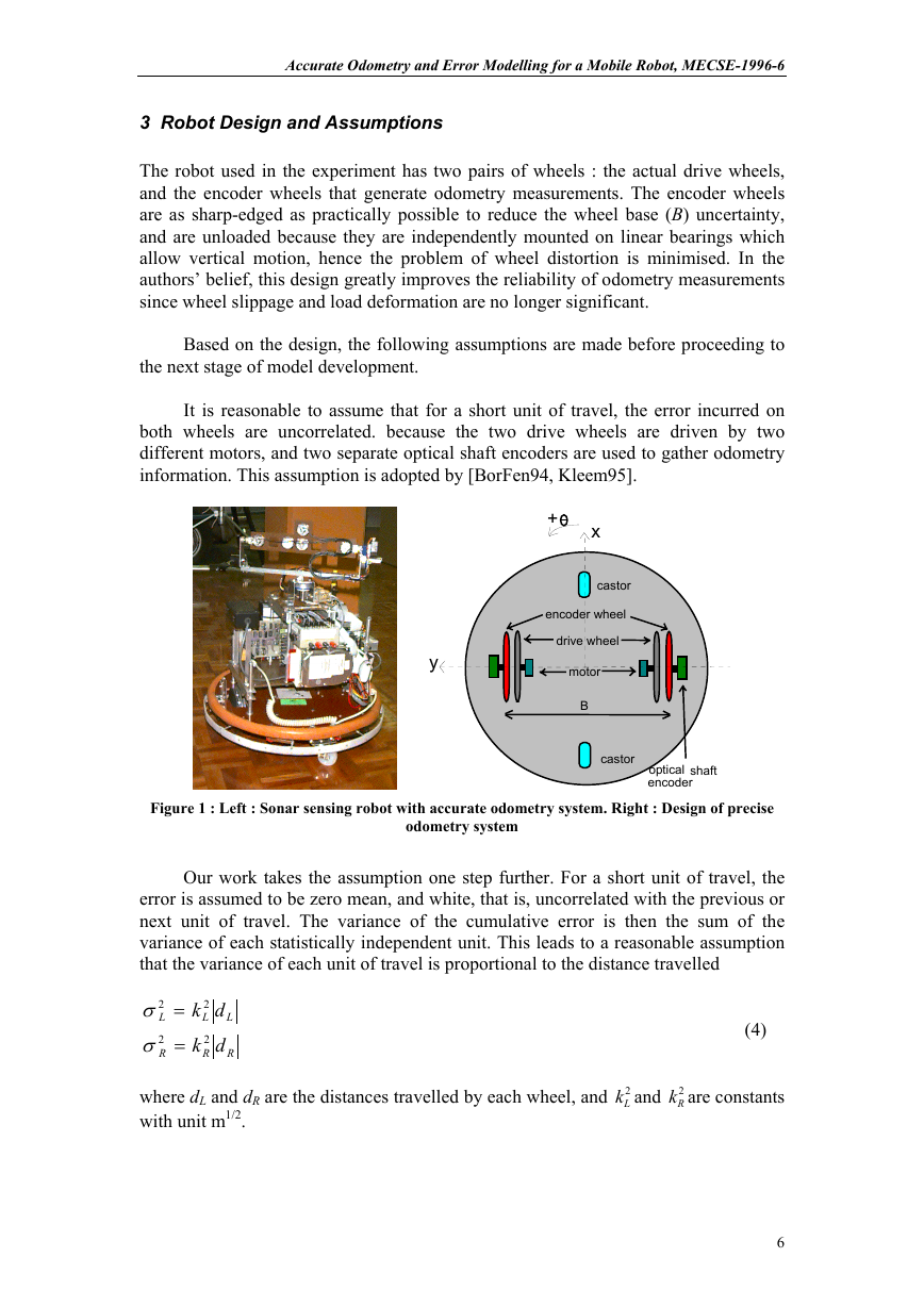
The robot used in the experiment has two pairs of wheels : the actual drive wheels,
and the encoder wheels that generate odometry measurements. The encoder wheels
are as sharp-edged as practically possible to reduce the wheel base (B) uncertainty,
and are unloaded because they are independently mounted on linear bearings which
allow vertical motion, hence the problem of wheel distortion is minimised. In the
authors’ belief, this design greatly improves the reliability of odometry measurements
since wheel slippage and load deformation are no longer significant.
Based on the design, the following assumptions are made before proceeding to
the next stage of model development.
It is reasonable to assume that for a short unit of travel, the error incurred on
both wheels are uncorrelated. because the two drive wheels are driven by two
different motors, and two separate optical shaft encoders are used to gather odometry
information. This assumption is adopted by [BorFen94, Kleem95].
+
x
castor
encoder wheel
drive wheel
motor
B
castor
optical shaft
encoder
y
Figure 1 : Left : Sonar sensing robot with accurate odometry system. Right : Design of precise
odometry system
Our work takes the assumption one step further. For a short unit of travel, the
error is assumed to be zero mean, and white, that is, uncorrelated with the previous or
next unit of travel. The variance of the cumulative error is then the sum of the
variance of each statistically independent unit. This leads to a reasonable assumption
that the variance of each unit of travel is proportional to the distance travelled
2
σ
L
2
σ
R
where dL and dR are the distances travelled by each wheel, and
with unit m
are constants
k d
2
L
k d
2
R
and
=
=
L
R
kL
2
kR
2
1/2.
(4)
6
�
Accurate Odometry and Error Modelling for a Mobile Robot, MECSE-1996-6
4 Calibration of Systematic Error Using UMBmark Test
UMBmark test [BorFen94] has been used for the calibration of wheel base error and
unequal wheel diameter error. The principles and mathematical details of the
procedures can be found in [BorFen94] so only key equations are summarised here. In
short, the robot was programmed to travel a square path of side D in the clockwise
sense (CW) for a number of times, say n, and the offsets of the final Cartesian
coordinates from the initial Cartesian coordinates, exi,CW, eyi,CW were recorded. The
experiment was repeated for the counterclockwise sense (CCW) and exi,CCW, eyi,CCW
were recorded. The ‘tuning factors’ required to be incorporated into the software to
counteract the effect of the systematic errors have been calculated from the weighted
Cartesian offsets in both senses. As summary, the centres of gravity of the offsets can
be computed from the their averages
x
c g CW CCW
.
i CW CCW
,
(5)
ex
=
n
n
.,
/
/
y
c g CW CCW
.
.,
/
=
ey
i CW CCW
,
/
(6)
With the two pairs of centres of gravity, the tuning factors for the wheel base,
the radius of left wheel and the radius of right wheel, cb, cl and cr, can be found by
following this sequence of computations:
∑1
i
1
=
n
∑1
n
i
1
=
.,
.,
x
+
c g CW
.
4
−
x
−
c g CW
.
4
−
2
)
2
)
average
average
D B
/
sin(
β
D B
sin(
/
β
)
−π π α/ (
)+1
+
−
α=
β=
E
d =
cb =
c
l
c
r
E
d
= 2 / (
E c
=
d l
.,
x
c g CCW
.
D
x
c g CCW
.
D
.,
,
,
.,
y
−
c g CW
.
4
−
y
+
c g CW
.
4
−
.,
.,
y
c g CCW
.
D
y
c g CCW
.
D
.,
(7)
(8)
(9)
(10)
(11)
(12)
and finally, the measure of dead-reckoning accuracy for systematic errors has been
defined in [BorFen94] as
E
max,
x
2
c g CCW
.
y
2
c g CCW
.
x
2
c g CW
.
y
2
c g CW
.
(13)
syst
+
=
+
,
.,
.,
.,
.,
(
max
)
5 The New Non-systematic Error Model
With the new non-systematic error model, the entire path travelled by the robot
is treated as consisting of k small segments. Propagation of error covariance is
required to be done k times to obtain the error covariance of the final state. This
section shows that it is possible to obtain a closed form solution for this model, as k
approaches infinity. The solution for a general circular arc motion is first developed.
7
�
Accurate Odometry and Error Modelling for a Mobile Robot, MECSE-1996-6
The solutions for two special cases, straight line motion and on-spot turn are then
obtained by suitably taking limits.
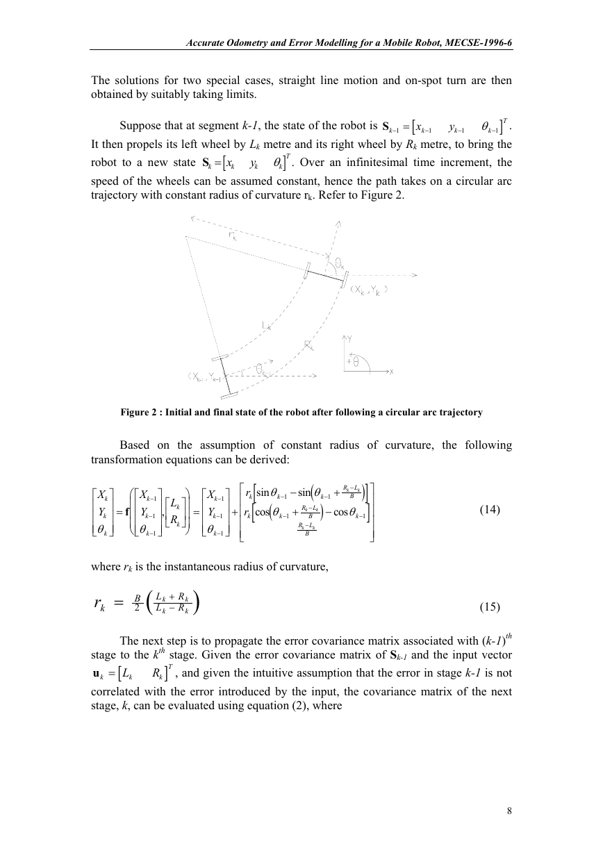
Suppose that at segment k-1, the state of the robot is
.
It then propels its left wheel by L
k metre and its right wheel by Rk metre, to bring the
robot to a new state S
y
. Over an infinitesimal time increment, the
k
k
speed of the wheels can be assumed constant, hence the path takes on a circular arc
trajectory with constant radius of curvature r
k. Refer to Figure 2.
1 θ
k
−
]
θ
k
=1
−
y
k
x
k
S
=
x
[
]
[
1
−
1
−
T
T
k
k
Figure 2 : Initial and final state of the robot after following a circular arc trajectory
Based on the assumption of constant radius of curvature, the following
rk
=
B
2
)
(
L
L
k
k
+
−
R
R
k
k
(15)
[
=
L
k
The next step is to propagate the error covariance matrix associated with (k-1)th
stage to the kth stage. Given the error covariance matrix of Sk-1 and the input vector
uk
, and given the intuitive assumption that the error in stage k-1 is not
correlated with the error introduced by the input, the covariance matrix of the next
stage, k, can be evaluated using equation (2), where
R
k
]
T
8
k
k
f
1
−
=
transformation equations can be derived:
X
Y
k
θ
k
where rk is the instantaneous radius of curvature,
(
sin
−
θ
k
)
R L
−
+
k
k
B
R L
−
k
k
B
[
sin
θ
k
1
−
[
(
cos
θ
k
r
k
r
k
X
Y
k
θ
k
X
Y
k
θ
k
,
L
k
R
k
1
−
−
=
+
1
−
1
−
1
−
1
−
1
−
1
−
k
+
cos
R L
−
k
k
B
θ
k
]
)
]
1
−
(14)
�


 2023年江西萍乡中考道德与法治真题及答案.doc
 2012年重庆南川中考生物真题及答案.doc
 2013年江西师范大学地理学综合及文艺理论基础考研真题.doc
 2020年四川甘孜小升初语文真题及答案I卷.doc
 2020年注册岩土工程师专业基础考试真题及答案.doc
 2023-2024学年福建省厦门市九年级上学期数学月考试题及答案.doc
 2021-2022学年辽宁省沈阳市大东区九年级上学期语文期末试题及答案.doc
 2022-2023学年北京东城区初三第一学期物理期末试卷及答案.doc
 2018上半年江西教师资格初中地理学科知识与教学能力真题及答案.doc
 2012年河北国家公务员申论考试真题及答案-省级.doc
 2020-2021学年江苏省扬州市江都区邵樊片九年级上学期数学第一次质量检测试题及答案.doc
 2022下半年黑龙江教师资格证中学综合素质真题及答案.doc