Theoretical Economics Letters, 2020, 10, 299-304
https://www.scirp.org/journal/tel
ISSN Online: 2162-2086
ISSN Print: 2162-2078
Why Individual Behavior Is Key to the Spread of
Viruses Such as Covid-19
Michael Grabinski, Galiya Klinkova
Department of Business and Economics, Neu-Ulm University, Wileystr, Neu-Ulm, Germany
How to cite this paper: Grabinski, M., &
Klinkova, G. (2020). Why Individual Beha-
vior Is Key to the Spread of Viruses Such as
Covid-19. Theoretical Economics Letters,
10, 299-304.
https://doi.org/10.4236/tel.2020.102020
Received: February 22, 2020
Accepted: April 20, 2020
Published: April 23, 2020
Copyright © 2020 by author(s) and
Scientific Research Publishing Inc.
This work is licensed under the Creative
Commons Attribution International
License (CC BY 4.0).
http://creativecommons.org/licenses/by/4.0/
Open Access
Abstract
Diseases are spread due to the behavior of people. One may have millions of
differently behaving people. For simplicity, humankind is only considering
the average behavior. However, this simplification can lead to results tre-
mendously different from the exact solution in at least some applications
when non-linear differential equations are used. In this letter, we prove that
the mistake is very big for the spread of infections like Covid-19. Ten percent
ignoring the rules can almost ruin the extremely careful behavior of the re-
maining ninety percent. This is totally different to most business situations
where considering eighty percent is sufficient (“80-20-rule”). This may ex-
plain why the spread of the Covid-19 pandemic and the impact of measures
against it are hard to predict for decision makers.
Keywords
Covid-19, Disease Spread, Average, Non-Linear Differential Equations, Chaos
1. Introduction
Any growth rate, be it population growth or the spread of a virus infection, is
exponential in the beginning. Because nothing is infinite, there will be some sa-
turation. There is a variety of models which are very similar at least for the ef-
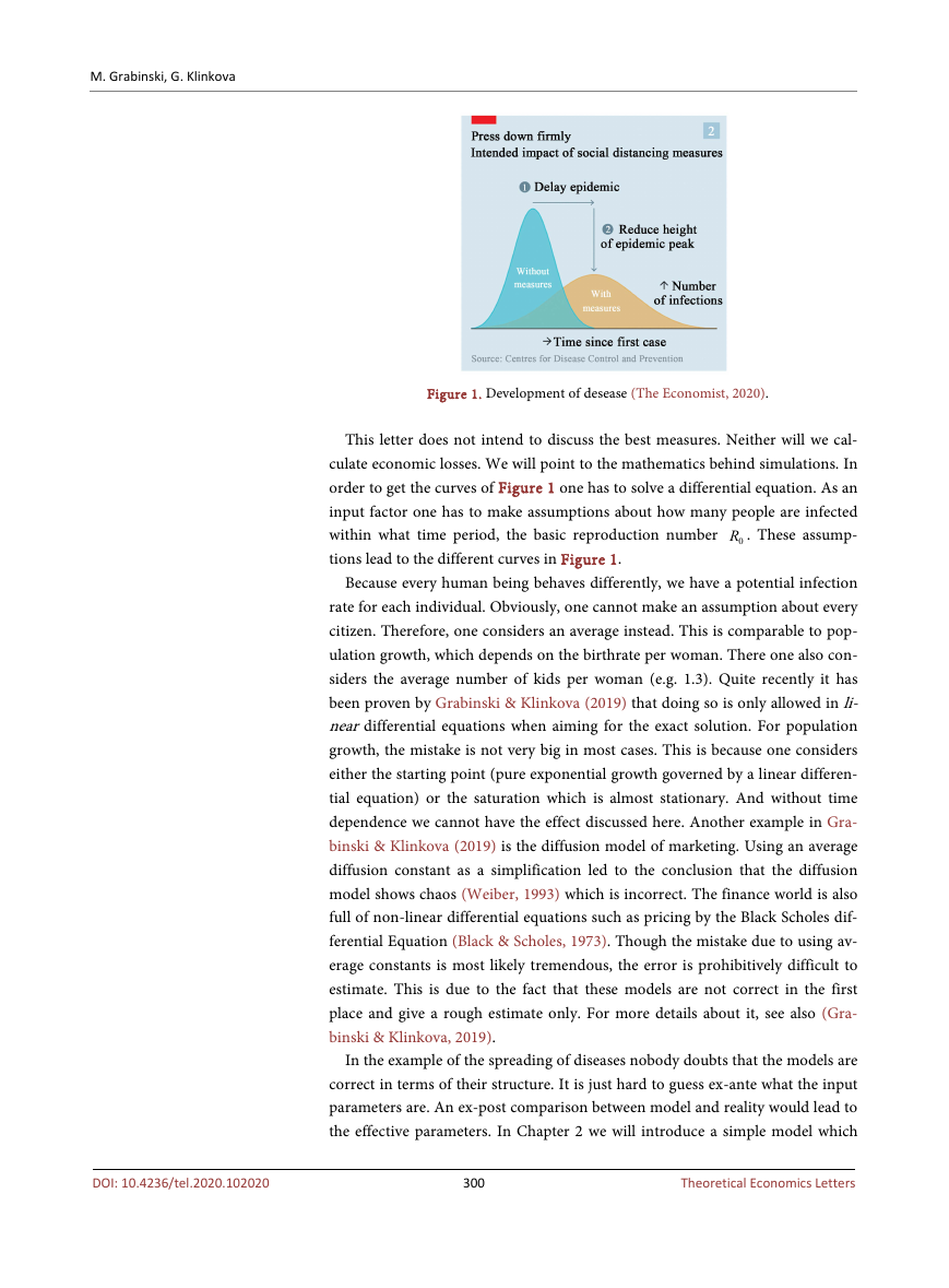
fects discussed here. They are also used to create charts like Figure 1. In this
case, we see the development for the spread of Covid-19 over time. It can be-
come narrow and high (all cases within a short time span) or wide and low (cas-
es are spread over a long time). Though the total number of cases stays the same,
the latter one is more desirable. Hospitals can handle the second scenario much
better. Economically speaking it is easier to bear some losses over two years for
example, rather than a catastrophe within three months. The obvious measures
to obtain the second scenario are to ensure people to behave carefully.
DOI: 10.4236/tel.2020.102020 Apr. 23, 2020
299
Theoretical Economics Letters
�
M. Grabinski, G. Klinkova
Figure 1. Development of desease (The Economist, 2020).
This letter does not intend to discuss the best measures. Neither will we cal-
culate economic losses. We will point to the mathematics behind simulations. In
order to get the curves of Figure 1 one has to solve a differential equation. As an
input factor one has to make assumptions about how many people are infected
within what time period, the basic reproduction number
0R . These assump-
tions lead to the different curves in Figure 1.
Because every human being behaves differently, we have a potential infection
rate for each individual. Obviously, one cannot make an assumption about every
citizen. Therefore, one considers an average instead. This is comparable to pop-
ulation growth, which depends on the birthrate per woman. There one also con-
siders the average number of kids per woman (e.g. 1.3). Quite recently it has
been proven by Grabinski & Klinkova (2019) that doing so is only allowed in li-
near differential equations when aiming for the exact solution. For population
growth, the mistake is not very big in most cases. This is because one considers
either the starting point (pure exponential growth governed by a linear differen-
tial equation) or the saturation which is almost stationary. And without time
dependence we cannot have the effect discussed here. Another example in Gra-
binski & Klinkova (2019) is the diffusion model of marketing. Using an average
diffusion constant as a simplification led to the conclusion that the diffusion
model shows chaos (Weiber, 1993) which is incorrect. The finance world is also
full of non-linear differential equations such as pricing by the Black Scholes dif-
ferential Equation (Black & Scholes, 1973). Though the mistake due to using av-
erage constants is most likely tremendous, the error is prohibitively difficult to
estimate. This is due to the fact that these models are not correct in the first
place and give a rough estimate only. For more details about it, see also (Gra-
binski & Klinkova, 2019).
In the example of the spreading of diseases nobody doubts that the models are
correct in terms of their structure. It is just hard to guess ex-ante what the input
parameters are. An ex-post comparison between model and reality would lead to
the effective parameters. In Chapter 2 we will introduce a simple model which
300
Theoretical Economics Letters
DOI: 10.4236/tel.2020.102020
�
M. Grabinski, G. Klinkova
produces curves like the one of Figure 1. However, the outcome is strikingly
different whether one takes an average infection rate or a varying one. Assume
that if everybody in the population behaved carefully, this would lead to a spread
of the disease over e.g. 24 months, while if everybody behaved badly, the disease
would spread over three months only, for instance. If we assume that half of the
population behaves badly and the other half is extremely careful, it may be a
quite reasonable behavior on average. This average would lead to a spread of the
disease over 24 months if everybody shows this behavior. However, the actions
of the badly behaving half will lead to a spread of the disease over little more
than three months in total. Because the spread is exponential rather than linear,
the extremely careful half will be infected by the badly behaving with almost no
delay making their effort worthless.
In Chapter 3 we will draw conclusions. Instead of limiting the average number
of social contacts in order to curb the spread of Covid-19, one has to make sure
that almost everybody takes a minimum of caution.
2. Growth Model
As one gets from almost all mathematical textbooks (e.g. Bronshtein et al., 2007)
a population
will grow proportionally to n:
( )n t
( )
n t
1
= ⋅
τ
( )
n t
(1)
Equation (1) will lead to unlimited growth. The constant 1 τ is the speed. A
small τ will lead to rapid growth, a big one to slow growth. In the case of the
spread of diseases, τ can be estimated by the reproduction number
0R . But
this is not our goal here. We are just assuming different values of τ for differ-
ent parts of the population.
Of course, the unlimited growth of Equation (1) holds only in the beginning.
In the case of Covid-19 experts reckon that about two thirds of the population
will get infected eventually without vaccination. In order to stay general, we
normalize the part of the population being infected eventually to 1. For example
for Germany, with roughly 80 million inhabitants and about 50 million potential
infections, this means that in case of 1000 infected people n takes a value of
5
. There are various approaches to put a limit on Equation (1). The sim-
2 10−×
plest is a limitation borrowed from the logistic equation:
( )
n t
=
1
τ
⋅
( )
n t
⋅
(
1
−
( )
n t
)
(2)
This approach is not untypical for growth limitations. When
ap-
proaches its maximum 1, growth becomes slower and slower. The solution of
Equation (2) can be given in a closed form:
e
n
⋅
0
(
1
n
− −
0
(3)
( )
n t
t
e
1
=
( )n t
t
τ
)
⋅
τ
DOI: 10.4236/tel.2020.102020
In order to get curves like the one of Figure 1 one has to take the derivative
Theoretical Economics Letters
301
�
M. Grabinski, G. Klinkova
with respect to time of Equation (3):
( )
n t
=
n
0
τ
⋅
t
e
(
+
τ
t
e
(
1
τ
−
−
)
n
0
)
1
n
0
(
1
2
)
(4)
5
2 10−×
infections as the starting value
A presumably very similar formula has been used to produce the curves of
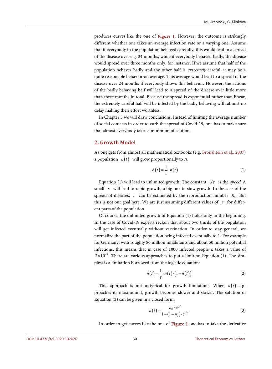
Figure 1. We now plot Equation (4) for three different values of τ. We always
took
0n . The time units are arbitrary.
One may think of months. Then the first society (blue curve, tallest) has every-
body infected within under one year, the second (orange curve) in about two
years and the third (green curve, smallest) within over three years. The curves of
Figure 2 are the results for three societies behaving differently. If half of the so-
ciety behave like in the blue curve and the other half like in the green curve, one
may naively conclude that the whole society will get infections over time like in
the orange curve. Unfortunately, this is not true. The people from the blue curve
will infect the people from the green curve much earlier than the people of the
green curve would do if they were alone. Assuming that the careful ones of the
society will not infect so many people but were also infected equally by the care-
less people, one will get two coupled differential equations:
n
1
+
n
2
=
n
1
τ
1
(
1 2
⋅ −
n
1
)
+
n
2
τ
2
(
1 2
⋅ −
n
2
)
n
n=
(5)
2
1
( )
n t
The indices 1 and 2 refer to the two halves of the society.
( )
n t
2
is the entire society. The first equation in Equation (5) states the infection rate of
the entire population
. Both population groups have the limit 1/2. The
second equation states that both halves of population are infected equally. Of
course one can modify this. One can also generalize Equation (5) so that the two
parts of the population are not equal in size. Equation (6) is valid when only ten
percent are in group 1 and ninety percent are in group 2:
( )
n t
1
n
1
n+
2
=
+
n
1
+
n
2
=
n
1
τ
1
(
1 10
⋅ −
)
n
1
+
n
2
τ
2
1
⋅ −
10
9
n
2
9n
n=
(6)
2
1
Figure 2. Plot of Equation (4) for τ = 0.5, 1.5, and 2.5.
302
Theoretical Economics Letters
DOI: 10.4236/tel.2020.102020
�
M. Grabinski, G. Klinkova
( )n t
=
5
−
. Blue curve from Equation
= ×
18 10
2 10
6
n−
02
.
=
×
6
−
=
n
02
n
01
with
τ =
2
, and orange curve from Equation (6),
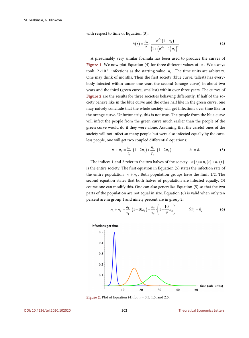
Figure 3. Total infections
(5),
The factors in Equation (6) are chosen so that the ratio of
2.5
n
01
and
τ =
1
0.5
10
1n to
2n is 1 to 9.
Equations (5) or (6) are integrable. But the result cannot be written down in a
closed form. We have therefore chosen to solve Equations (5) and (6) numeri-
cally. In Figure 3, we have plotted the solution of Equation (5) in the blue curve.
The result is only slightly different from the blue curve in Figure 2. If half of the
population behaves like in the blue curve of Figure 2 and half like the green
curve, it is only slightly better compared to the situation where all people behave
like the blue curve in Figure 2. The effort of the very careful ones is (almost)
wasted. Even if ninety percent are behaving very carefully (orange curve in Fig-
ure 3), we are only slightly better off than the orange curve in Figure 2.
3. Conclusions and Further Work
We have shown that the bad behavior of one half cannot be compensated by the
very good behavior of the other half in order to reach the goal of spreading cases
of a disease over a long period. We have a situation where a very broad majority
must take appropriate measures as otherwise measures become effectless. As we
see from the orange curve in Figure 3, ten percent can tremendously change the
outcome for everybody though ninety percent show a perfect behavior. It is
therefore not enough that politicians look to a broad majority. They have to
scrutinize the ten percent ignoring the pandemic.
A final discussion with real numbers is only possible after the pandemic. But
even today the findings of this letter may (partly) explain why European coun-
tries are hit so differently. The culture of obeying rules is very different in dif-
ferent countries.
As an extension to this work one may use a distribution of behavior instead of
just two values for τ. However, this leads to extremely complicated mathemat-
ics, but most likely does not change results much.
Having non-linear differential equations one may also look for chaos, see e.g.
Schuster, 1984. Equations (5) and (6) will (most likely) never show chaos in
Theoretical Economics Letters
303
DOI: 10.4236/tel.2020.102020
�
M. Grabinski, G. Klinkova
themselves. However, changing the model at a certain point may have dramatic
effects. In Equations (5) or (6) it would mean changing the τ at a certain point
in time. Politically speaking it means taking a certain measure such as a curfew
earlier or later. In doing so chaos effects are likely. Such chaos effects are more
like “the drop of honey effect” as defined in Filipe & Ferreira, 2013 (see also
Filipe et al., 2010) in contrast to chaos effects like in the weather forecast.
Furthermore, people often speak of panic in the current Covid-19 pandemic.
A panic is an abrupt change of behavior. In our model, it is a (discontinuous)
change in τ or the ratio of
2n . In doing so chaos effects are very likely.
This might be a good quantification of the above mentioned “drop of honey ef-
fect.”
1n to
Conflicts of Interest
The authors declare no conflicts of interest regarding the publication of this pa-
per.
References
Black, F., & Scholes, M. (1973). The Pricing of Options and Corporate Liabilities. Journal
of Political Economy, 81, 637-654. https://doi.org/10.1086/260062
Bronshtein, I. N., Semenddyayev, K. A., Musiol, G., & Muehlig, H. (2007). Handbook of
Mathematics (5th English Edition). Berlin Heidelberg: Springer.
Filipe, J. A., & Ferreira, M. A. M. (2013). Social and Political Events and Chaos Theory:
The “Drop of Honey Effect”. Emerging Issues in the Natural and Applied Sciences, 3,
126-137.
Filipe, J. A., Ferreira, M. A. M., Coelho, M., & Pedro, M. I. (2010). Chaos, Anti-Chaos and
Resources: Dealing with Complexity. Journal of Applied Mathematics, 3, 83-90.
Grabinski, M., & Klinkova, G. (2019). Wrong Use of Averages Implies Wrong Results
from Many Heuristic Models. Applied Mathematics, 10, 605-618.
https://doi.org/10.4236/am.2019.107043
Schuster, H. G. (1984). Deterministic Chaos. Physik Verlag, Weinheim.
The Economist (2020). Briefing Covid19, Feb. 29, 2020, 15.
https://www.economist.com/briefing/2020/02/29/covid-19-is-now-in-50-countries-and
-things-will-get-worse
Weiber, R. (1993) Chaos: Das Ende der klassischen Diffusionsmodellierung? Marketing
ZFP, 1, 35-46. https://doi.org/10.15358/0344-1369-1993-1-35
DOI: 10.4236/tel.2020.102020
304
Theoretical Economics Letters
�



 2023年江西萍乡中考道德与法治真题及答案.doc
 2012年重庆南川中考生物真题及答案.doc
 2013年江西师范大学地理学综合及文艺理论基础考研真题.doc
 2020年四川甘孜小升初语文真题及答案I卷.doc
 2020年注册岩土工程师专业基础考试真题及答案.doc
 2023-2024学年福建省厦门市九年级上学期数学月考试题及答案.doc
 2021-2022学年辽宁省沈阳市大东区九年级上学期语文期末试题及答案.doc
 2022-2023学年北京东城区初三第一学期物理期末试卷及答案.doc
 2018上半年江西教师资格初中地理学科知识与教学能力真题及答案.doc
 2012年河北国家公务员申论考试真题及答案-省级.doc
 2020-2021学年江苏省扬州市江都区邵樊片九年级上学期数学第一次质量检测试题及答案.doc
 2022下半年黑龙江教师资格证中学综合素质真题及答案.doc