Modern Economy, 2020, 11, 407-425
https://www.scirp.org/journal/me
ISSN Online: 2152-7261
ISSN Print: 2152-7245
Research on Pricing of Shanghai 50ETF Options
Based on Fractal B-S Model and GARCH Model
Wanting Hu
School of Econmics, Jinan University, Guangzhou, China
How to cite this paper: Hu, W. T. (2020).
Research on Pricing of Shanghai 50ETF
Options Based on Fractal B-S Model and
GARCH Model. Modern Economy, 11,
407-425.
https://doi.org/10.4236/me.2020.112031
Received: December 20, 2019
Accepted: February 17, 2020
Published: February 20, 2020
Copyright © 2020 by author(s) and
Scientific Research Publishing Inc.
This work is licensed under the Creative
Commons Attribution International
License (CC BY 4.0).
http://creativecommons.org/licenses/by/4.0/
Open Access
Abstract
A reasonable option trading price will have certain guiding significance for
option traders. Fractal B-S model and GARCH model are common pricing
methods. This article explores which pricing method is more reasonable
based on SSE 50ETF options. Due to the spikes and thick tails, conditional
heteroscedasticity, and fractal characteristics of the SSE 50ETF option yield
data, this paper performs stationary test, autocorrelation and partial autocor-
relation test, ARCH test, and Hurst test on the daily sample rate series of the
target sample. The characteristics of the yield sequence are used to construct a
GARCH model and predict the daily rate of volatility. Finally, the volatility
predicted by the GARCH model is used as the parameter value in the fractal
Brownian motion option pricing method to realize the option pricing. At the
same time, this paper calculates the pricing results of the BS option pricing
method based on historical volatility, and compares the two options pricing
results with the closing price of the option transaction price. The results show
that the prediction of the Shanghai Securities 50ETF option pricing method
based on the GARCH fractal Brownian motion model. The accuracy is sig-
nificantly higher than the standard BS option pricing method.
Keywords
Fractal Brownian Motion, GARCH Model, SSE 50ETF Options, Volatility
Prediction, Improved B-S European Option Pricing
1. Introduction
1.1. Background and Significance of Topic Selection
The full name of the SSE 50 ETF is the SSE 50 Trading Open-end Index Securi-
ties Investment Fund, which was established on December 30, 2014, and is the
first ETF product in Mainland China. The SSE 50ETF is a completely passive
DOI: 10.4236/me.2020.112031 Feb. 20, 2020
407
Modern Economy
�
W. T. Hu
DOI: 10.4236/me.2020.112031
index fund. It completely replicates the constituent stocks of the SSE 50 Index
and the weight of each constituent stock. Its investment income comes from the
SSE 50 Index. On February 9, 2015, the Shanghai Stock Exchange launched the
Shanghai Securities 50ETF as the underlying trading option, namely the Shang-
hai Securities 50ETF option. The launch of this option has not only enriched
China’s financial derivative products, but also marked a key step in the devel-
opment of the option derivative market in China; it has also achieved a joint de-
velopment of the current market, improved the operating efficiency of the spot
market, and further enhanced the ability to serve the real economy. Option
pricing is one of the important contents of modern financial theory. Reasona-
bly pricing options are the prerequisite for options to play their important role
in the financial market. It has important practical significance for China to
further develop derivatives, avoid risks, and stabilize financial markets. How to
effectively establish the SSE 50ETF option pricing model is also an important
topic.
Although the development of options in China started late, some scholars
have conducted research on option pricing. Ji (2015) used the GARCH model
and the B-S model to analyze the SSE 50ETF option price, and concluded that
the GARCH model has a good fitting effect on small sample data. Liu et al.
(2018) conducted European barrier option pricing research in a mixed-fraction
Brownian motion environment, and derived the European barrier option call
put-parity relationship, and then entered the knockout option relationship to
introduce all types of barrier option pricing formulas. Cheng et al. (2018) consi-
dered the pricing of European options when paying continuous dividends under
the sub-fractional Brownian motion environment, and estimated the parameters
in the pricing model. The unbiasedness and strong convergence of the estima-
tors were discussed. It can be seen that both the fractal Brownian motion model
and the B-S model are common method models for studying option pricing
methods. In this paper, the Shanghai 50ETF is the research object. Based on the
comparison between the pricing of the two models and historical actual condi-
tions, which model is selected as a more reasonable pricing model.
1.2. Comparison between Traditional B-S Option Pricing Method
and Fractal Brownian Motion Option Pricing Method
The B-S option pricing method is proposed under the assumption that the un-
derlying asset prices are independent of each other and follow the geometric
Brownian motion, and that the return on the underlying asset is independent
and identically distributed and follows the normal distribution. However, in re-
cent years, a large number of scholars’ research on the capital market has shown
that the price of financial assets does not follow the geometric Brownian motion,
that is, the rate of return of financial assets does not follow a normal distribu-
tion, but a distribution of peaks and thick tails. It is not independent, but there is
long-term correlation. Therefore, the B-S option pricing method has some limi-
tations in practical application.
408
Modern Economy
�
W. T. Hu
The fractal Brownian motion option pricing method is the first time that Hu
Y applied it to financial option pricing based on Mandelbrot B’s fractal Brow-
nian motion. The main difference between fractal Brownian motion and geome-
tric Brownian motion is that the increment in fractal Brownian motion is not
independent, while the increment in geometric Brownian motion is indepen-
dent. Because the fractal Brownian motion option pricing method can well cha-
racterize the self-similarity, thick tail, and long memory of the underlying asset
price, and does not require the underlying asset prices to be independent of each
other, obey the geometric Brownian motion, and the underlying asset return rate
to follow a normal distribution Therefore, it is more in line with the actual cha-
racteristics of financial option prices. Subsequently, many researchers used the
fractal Brownian motion option pricing method to study the pricing problem of
the stock option market under the assumption that the stock price volatility was
constant. It was verified that the fractal Brownian motion option pricing method
was superior to B-S and other option pricing methods.
2. Literature Review
2.1. Literature Review of Volatility Models at Home and Abroad
There are many researches on the modeling and prediction methods of volatility.
Robert Engle proposed an autoregressive conditional heteroscedasticity (ARCH)
model in 1982 to build and predict conditional heteroscedasticity models. Early
ARCH family models include ARCH-M models, TARCH and NARCH models.
The ARCH-M model was first proposed by Engle, Robins, and Lilien in 1985.
The ARCH model takes into account the variation of conditional variance over
time to analyze volatility, and the analysis of volatility is inseparable from the
risk. Engle et al. further took into consideration the important use of conditional
variance as a risk measure that changes over time, linking risk and return, and
proposed the ARCH-M model, which allows conditional heteroscedasticity to
directly affect the mean of returns. The TARCH model considers the variance is
affected by the sign of the disturbance term, and NARCH is an important non-
linear ARCH model. Both of them specifically address some of the defects of the
linear ARCH model, which is more than the linear ARCH model advanced.
However, in some cases, the ARCH model cannot express the information that
the autocorrelation coefficient is slowly decaying, and in practice, the estimation
of the completely free lag distribution often leads to the destruction of
non-negative constraints. To solve the shortcomings of the ARCH model, Bol-
lerslev (1986) proposed the GARCH model in 1986. The variance of the random
disturbance term is not only related to the variance of the lagging disturbance
term, but also to the lagging disturbance term itself. After that, the EGARCH
(Exponential GARCH) model was proposed by Nelson in 1991. The biggest ad-
vantage of the model is that it takes the form of the logarithm of conditional va-
riance, which allows the assumption of the sum of the squared residuals and the
409
Modern Economy
DOI: 10.4236/me.2020.112031
�
W. T. Hu
DOI: 10.4236/me.2020.112031
conditional variance to be more advanced. Flexible to capture asymmetric con-
ditions (good news and bad news have asymmetric market volatility). China’s
financial derivatives industry started late, and there are few innovative studies on
volatility using the GARCH family, and more emphasis is placed on applica-
tions. Representative examples are Zheng and Huang (2010). The comparison of
the prediction capabilities of the GARCH model and the implied volatility is
mainly based on the research on the volatility of the Hong Kong Hang Seng In-
dex Options Market. There are more information and strong forecasting ability;
but when forecasting for a long period of time, the implied volatility contains
more information and strong forecasting ability. At the same time, the more ac-
tive the options market transactions, the more comprehensive the information it
reflects, and the stronger the ability to predict implied volatility. In addition,
Huang and Zhong (2007) also evaluated the volatility prediction of GARCH
models. The research results show that the GARCH model is used to compre-
hensively estimate the rate of return and out-of-sample prediction. The use of
M-Z regression and loss function shows that it performs very well and can per-
form better predictions.
The study of volatility can reflect the market’s expectations of the degree of
future volatility, thereby achieving the purpose of risk prevention and guiding
transactions. For example, in 1993 the Chicago Board Options Exchange com-
piled the VIX Volatility Index based on the S & P Index. To this day, the volatil-
ity index has become the main reference indicator for measuring investor psy-
chology and market volatility. It uses stock index option prices to calculate ex-
pected short-term market volatility. The volatility index can not only quantify
the price changes of derivatives and market risks, but also provides investment
opportunities due to its volatile nature. The market can make full use of its cha-
racteristics to develop tradable volatility products for hedged trading and arbi-
trage trading.
Research on volatility can give investors a better understanding of risk. At
present, domestic stock index options are only listed and traded on the Shanghai
Stock Exchange 50ETF options. The study of volatility can lay the foundation for
the subsequent listing of more financial options.
2.2. Literature Review on Options Pricing at Home and Abroad
Since 1970, on financial option pricing, Black-Scholes (BS) option pricing, Hull-
White option pricing, binary tree option pricing, and fractal Brownian motion
option pricing have emerged, among which BS option pricing and fractal Brown
Exercise option pricing are more common and easy-to-use methods.
With the development of the foreign option market, the empirical research on
option pricing has become more and more in-depth, mainly including the im-
provement of variables or parameters and the validation of models. The empiri-
cal start on the improvement of variables or parameters was the earliest. Levy
and Byun (1987) tried to test the reliability of BS model pricing by deriving the
410
Modern Economy
�
W. T. Hu
implied volatility of the price based on the confidence interval of the estimated
variance; Corrado and Su (1998) through empirical research on the S & P 500
stock index options, it is found that the return volatility is negatively correlated
with changes in the stock index level, and the parameters of the stochastic vola-
tility option pricing model are estimated and predicted, and the practical appli-
cation value of the stochastic volatility option pricing model is revealed. Saurab-
ha and Tiwari (2007) in order to solve the volatility smile problem in the tradi-
tional BS option pricing model, two statistical variables of skewness and kurtosis
are introduced. Based on the relevant data of S & P 500 options, the volatility is
used. Estimating the prices of deep currency options and deep out-of-the-money
options can produce prediction results that are closer to the market price of op-
tions; Andrés-Sánchez (2017) analyzes the option pricing model based on the
basic theory of the fuzzy BS model, through the actual trading of Spanish stock
index options Price fitting related parameters, fuzzy BS model from different an-
gles. The ability to predict the price of stock index options is evaluated. Regard-
ing the validity analysis of the model, scholars’ empirical evidence is based on
different theoretical models. Bailey and Stulz (1989) performed dynamic analysis
and empirical testing of stock index options based on stochastic interest rate op-
tion pricing models and stochastic volatility option pricing models, respectively;
Yung and Zhang (2003) used S & P 500 option data to model GARCH option
pricing models Multi-angle empirical analysis with the pricing effect of the tra-
ditional BS model, and found that the GARCH model performs better than the
traditional BS model in sample evaluation and sample prediction; Kim and Lee
(2013) proposed an estimate of volatility without arbitrage Rate model, using
KOSPI 200 index options to conduct empirical analysis of three indicators: in-
tra-sample pricing, out-of-sample pricing and hedging error, verifying the effec-
tiveness of the model in option pricing; Oliver and Li (2015) from the equili-
brium interest rate and consumption Based on the perspective of capital asset
pricing, based on the price data of European call options, a reasonable prediction
of the price jump time in the jump-diffusion option pricing model is realized to
clarify how the relevant parameters of the model affect the actual option pricing.
Domestic research on the options market started late. With the further open-
ing of the financial market, the options trading market has become more and
more active, and research on pricing models has become more common.
Early scholars’ empirical research mainly focused on the pricing analysis of
alternatives to domestic market options and the data simulation of foreign mar-
ket-related options. Song et al. (2013) by studying the game between transferable
bond trading terms, introducing game options and selecting domestic converti-
ble bonds for empirical analysis, the double reflection wall backward stochastic
pricing model has better price simulation and prediction effects; Liao et al.
(2013) selected the Korean stock index option KOSPI200 as the research object,
and used the fractional Brownian motion option pricing model to fit relevant
actual data, and conducted an empirical test on the accuracy and effectiveness of
411
Modern Economy
DOI: 10.4236/me.2020.112031
�
W. T. Hu
DOI: 10.4236/me.2020.112031
the model. Qin et al. (2019) based on the fractional BS model, taking into ac-
count the uncertainty of the financial market including randomness and ambi-
guity, using stochastic analysis, fractal theory, and fuzzy set theory to construct a
long memory characteristic of financial markets under uncertainty European
option pricing model. Wang et al. (2019) combined a Heston model and a 3/2
model to establish a two-factor 4/2 stochastic volatility model, using S & P 500
index option data for pricing analysis.
2.3. Research Status of SSE 50ETF Option Pricing
In 2015, the emergence of China’s first listed options on the Shanghai Stock Ex-
change 50 ETF options in the capital market has led to an explosive growth in
domestic discussions and research on options pricing models.
Gu and Dong (2015) used the Shanghai and Shenzhen 300 stock index futures
and the Shanghai 50ETF options as samples to analyze the correlation coeffi-
cients and deviations of volatility of dispersion trading, and then analyze the
trading risks of the option pricing model. Yu and Chen (2016) used the theoret-
ical framework of the B-S model to conduct an empirical analysis on the core
parameters of the five SSE 50ETF options, including the underlying asset price,
and made relevant recommendations for the supervisors from the perspective of
contract design and risk control. At this stage, many scholars have conducted
in-depth discussions on the pricing of SSE 50ETF options from multiple pers-
pectives. Gong and Zhuang (2016) combined the asymmetric real variable
high-order moment model characterizing the high-order moment characteristics
of asset prices and the Levy process to describe the pure jump phenomenon of
price changes, and constructed the Levy-NGARCHSK model; this model fully
reflects the financial. The asset price path continues to be biased and leveraged.
Under the assumption that the innovation term obeys the non-Gaussian Levy
distribution, the author compares the accuracy and efficiency of the numerical
integral Cosine method and the Monte Carlo simulation pricing method to the
pricing of SSE 50ETF options. Fang, Zhang, and Qiao (2017) conducted an em-
pirical comparative analysis of the performance of the B-S model and Monte
Carlo simulation method on the pricing of SSE 50ETF options. The results show
that the IGARCH model can better fit the volatility of the Shanghai Stock Ex-
change 50ETF than the traditional GARCH model. When the number of simula-
tions is 1000, the efficiency of the Monte Carlo method is consistently higher
than that of the BSM model. The accuracy of other Monte Carlo models is also
higher than the BSM model; both the BSM model and the Monte Carlo simula-
tion method can accurately and effectively simulate the price of the SSE 50ETF
option. Lei and Wu (2017) used the Tobit model to analyze the impact of the
underlying asset liquidity on the SSE 50ETF option price and explained the va-
lidity of the option pricing; Hao and Du (2017) fused the GARCH model and the
generalized hyperbolic distribution based on their respective advantages, a
GARCH-GH option pricing model based on the SSE 50ETF was established. The
412
Modern Economy
�
W. T. Hu
results show that the pricing results of the GARCH-GH model are closer to the
actual prices of the SSE 50ETF options than the BS model and the GARCH-
Gaussian model. Wang and Yang (2016) used the high frequency data of the
Shanghai 50ETF option to empirically analyze the pricing accuracy of a hybrid
log-normal option pricing model with time-varying volatility, and found that the
model was superior to the one with event volatility characteristics B-S improved
model. Wu, Zhao, Li, & Ma (2019) made in-depth research on option pricing
under time-varying risk aversion, and concluded that TVRA-SV option pricing
model has better data fitting effect than traditional CRA-SV option pricing
model, and can more fully characterize the volatility of the SSE 50ETF return
under the objective and risk-neutral measure. Wu, Li, & Ma (2019) conducted
an empirical test using a stochastic volatility model, showing that the random
volatility model can obtain significantly more accurate and stable pricing results
than the traditional constant volatility B-S model, both within and outside the
sample.
Based on previous studies, this article uses the GARCH model to fit and pre-
dict the return volatility of the Shanghai 50ETF; the predicted volatility is used
as the input value to substitute the fractal Brownian motion option pricing
method, and the traditional and improved B-S option pricing method is used
to estimate.
3. The Establishment of Theoretical Methods and Models
3.1. Forecast Method of Yield Volatility
When using the B-S model to price options, it is assumed that the volatility of
asset prices is a constant value, which is not consistent with the actual financial
market situation, and the volatility is time-varying. Therefore, scholars have
proposed a series of stochastic volatility models to improve the B-S model, hop-
ing to better characterize the characteristics of stochastic volatility. In summary,
there are two main types of stochastic volatility models. One is a continuous-
time stochastic volatility model (SV model), and the other is a discrete-time sto-
chastic volatility model (GARCH model). In financial practice operations,
transactions are performed discretely. The GARCH model describes discrete-
time economic situations and better reflects the actual situation of stock price
operations in practice.
The GARCH model is an improvement of Bollerslev’s autoregressive condi-
tional heteroskedasticity (ARCH) model. It has been widely used in the financial
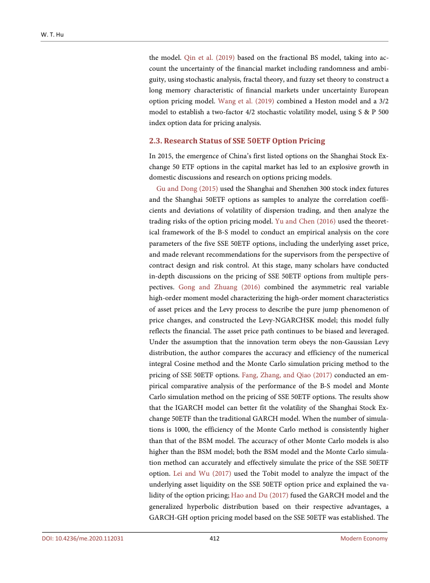
field since its creation. If the random variable y can be expressed as (1), u is said
to obey the q-order ARCH process.
x
1
t
−
2
u
σ β β
1
1
t
−
x
m t m
2
u
β
1
q t q
−
(2)
α α
1
+
0
=
(1)
−
+
x
2
t
2
u
β
2
t
−
α
2
+
+
+
u
t
+
α
y
t
=
+
−
+
+
0
2
t
2
DOI: 10.4236/me.2020.112031
Among them, since
2tσ− is the predicted value of the variance of the pre-
vious period based on the previous information, it is called the conditional va-
413
Modern Economy
�
W. T. Hu
riance. It can be seen from the above model that the variance of the noise at the
present moment is the regression of the square of the noise value of the finite
term in the past. On the one hand, it can be seen that the fluctuation of the noise
is affected by the previous period to produce memorability. The noise variance
at the past moments becomes larger and larger, and vice versa. In practical
terms, the overall level of volatility in the stock market in the previous period
will lead to a higher level of volatility in the current period, which forms the ag-
gregation and memory of the ARCH model. The probability density distribution
is spiked and thick-tailed.
Adding the lag of the residual squared to the conditional variance of Equation
=
(2) constitutes a GARCH model, as shown in Equation (3):
+
2
u
σ β β
1
1
t
−
+
β
2
0
2
u
β
Among them
1
1
t
−
2
χσ
is a GARCH term. Constraints are:
t p
−
2
+
2
χσ
1
1
t
−
2
χσ
1t
1
−
2
u
t
−
+
β
1
2
u
q t q
−
β
1
2
u
q t q
−
+
β
2
2
u
t
−
2
+
+
+
+
+
+
2
t
p
+
2
χσ
t p
−
p
(3)
is an ARCH term,
β
0
>
0;
β β
q
,
⋅⋅⋅
,
1
≥
0;
x
1
,
,
⋅⋅⋅
x
p
≥
0;
∑ ∑
β
i
+
x
j
<
1
q
i
1
=
p
j
1
=
The GARCH model believes that the variance of the error term in a certain
period depends not only on the variance of the error term with respect to time,
but also on the past error term itself. The model takes into account the lag value
of the disturbance term and the lag value of the conditional variance of the dis-
turbance term, which overcomes the ARCH model’s inability to reflect the per-
sistence of volatility, and is therefore widely used to describe the fluctuation of
asset returns in financial markets. However, the GARCH model still does not
solve the conditional heteroscedasticity in the early ARCH model, which de-
pends on the size of the random perturbation without considering the positive
and negative. This article does not discuss in depth.
A lot of empirical evidence shows that GARCH model has a good description
of financial time series. Therefore, this paper uses the GARCH model to predict
the volatility of SSE 50ETF returns. The prediction results are used as input val-
ues of the fractal Brownian motion model to price its options.
3.2. Fractal Brownian Motion Option Pricing Method
Geometric Brownian motion is an independent quantum process. It is a random
process with continuous time parameters and continuous state space. However,
the returns on financial assets are self-similar, thick-tailed, and long-memory.
The assumption of random walk in financial markets is not valid. For example,
some scholars found that the distribution of stock returns showed a “spike and
thick tail”. And the characteristics of the accumulation and persistence of vola-
tility, Mandelbrot (1968) also confirmed the fact that there is a “spike and thick
tail” in stock returns. Later many other scholars also revealed the fact that there
is a long-range correlation in financial market returns. When studied the obser-
vations of financial time series, they found that there was a significant autocor-
414
Modern Economy
DOI: 10.4236/me.2020.112031
�


 2023年江西萍乡中考道德与法治真题及答案.doc
 2012年重庆南川中考生物真题及答案.doc
 2013年江西师范大学地理学综合及文艺理论基础考研真题.doc
 2020年四川甘孜小升初语文真题及答案I卷.doc
 2020年注册岩土工程师专业基础考试真题及答案.doc
 2023-2024学年福建省厦门市九年级上学期数学月考试题及答案.doc
 2021-2022学年辽宁省沈阳市大东区九年级上学期语文期末试题及答案.doc
 2022-2023学年北京东城区初三第一学期物理期末试卷及答案.doc
 2018上半年江西教师资格初中地理学科知识与教学能力真题及答案.doc
 2012年河北国家公务员申论考试真题及答案-省级.doc
 2020-2021学年江苏省扬州市江都区邵樊片九年级上学期数学第一次质量检测试题及答案.doc
 2022下半年黑龙江教师资格证中学综合素质真题及答案.doc