算法导论第三版答案英文版.pdf-资料库

qq_29869043-9879764-4744302542978552638.pdf-第1页.png

第1页 / 共70页

qq_29869043-9879764-4744302542978552638.pdf-第2页.png

第2页 / 共70页

qq_29869043-9879764-4744302542978552638.pdf-第3页.png

第3页 / 共70页

qq_29869043-9879764-4744302542978552638.pdf-第4页.png

第4页 / 共70页

qq_29869043-9879764-4744302542978552638.pdf-第5页.png

第5页 / 共70页

qq_29869043-9879764-4744302542978552638.pdf-第6页.png

第6页 / 共70页

qq_29869043-9879764-4744302542978552638.pdf-第7页.png

第7页 / 共70页

qq_29869043-9879764-4744302542978552638.pdf-第8页.png

第8页 / 共70页

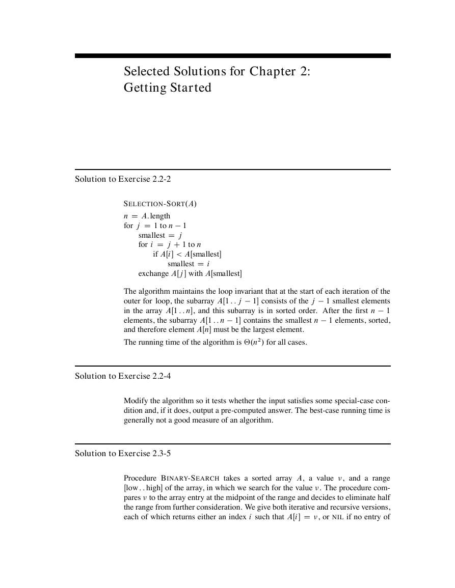
Selected Solutions for Chapter 2: Getting Started Solution to Exercise 2.2-2 SELECTION-SORT.A/ n D A:length for j D 1 to n 1 smallest D j for i D j C 1 to n if AŒi < AŒsmallest smallest D i exchange AŒj with AŒsmallest The algorithm maintains the loop invariant that at the start of each iteration of the outer for loop, the subarray AŒ1 : : j 1 consists of the j 1 smallest elements in the array AŒ1 : : n, and this subarray is in sorted order. After the ﬁrst n 1 elements, the subarray AŒ1 : : n 1 contains the smallest n 1 elements, sorted, and therefore element AŒn must be the largest element. The running time of the algorithm is ‚.n2/ for all cases. Solution to Exercise 2.2-4 Modify the algorithm so it tests whether the input satisﬁes some special-case con- dition and, if it does, output a pre-computed answer. The best-case running time is generally not a good measure of an algorithm. Solution to Exercise 2.3-5 Procedure BINARY-SEARCH takes a sorted array A, a value , and a range Œlow : : high of the array, in which we search for the value . The procedure com- pares to the array entry at the midpoint of the range and decides to eliminate half the range from further consideration. We give both iterative and recursive versions, each of which returns either an index i such that AŒi D , or NIL if no entry of

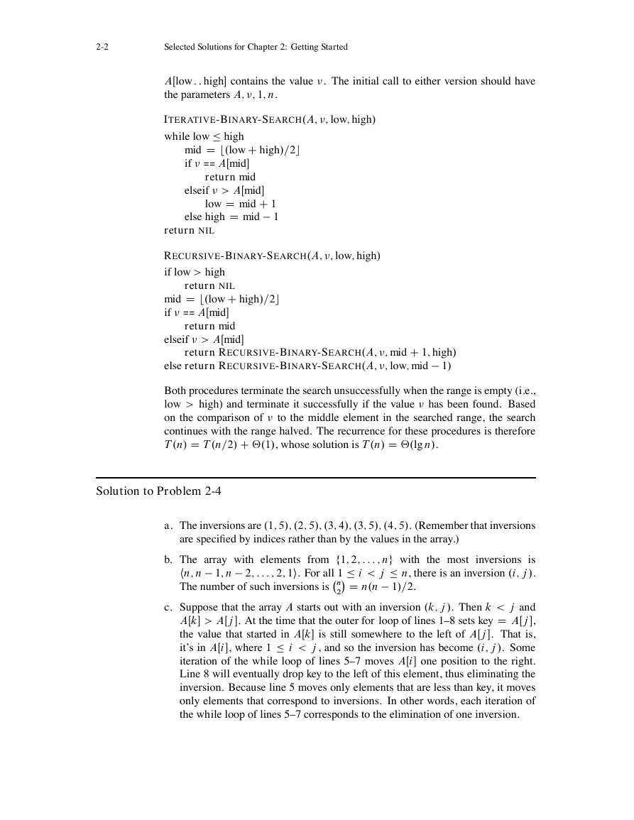
2-2 Selected Solutions for Chapter 2: Getting Started AŒlow : : high contains the value . The initial call to either version should have the parameters A; ; 1; n. ITERATIVE-BINARY-SEARCH.A; ; low; high/ while low high mid D b.low C high/=2c if == AŒmid return mid elseif > AŒmid low D mid C 1 else high D mid 1 return NIL RECURSIVE-BINARY-SEARCH.A; ; low; high/ if low > high return NIL mid D b.low C high/=2c if == AŒmid return mid elseif > AŒmid return RECURSIVE-BINARY-SEARCH.A; ; mid C 1; high/ else return RECURSIVE-BINARY-SEARCH.A; ; low; mid 1/ Both procedures terminate the search unsuccessfully when the range is empty (i.e., low > high) and terminate it successfully if the value has been found. Based on the comparison of to the middle element in the searched range, the search continues with the range halved. The recurrence for these procedures is therefore T .n/ D T .n=2/ C ‚.1/, whose solution is T .n/ D ‚.lg n/. Solution to Problem 2-4 a. The inversions are .1; 5/; .2; 5/; .3; 4/; .3; 5/; .4; 5/. (Remember that inversions are speciﬁed by indices rather than by the values in the array.) b. The array with elements from f1; 2; : : : ; ng with the most inversions is hn; n 1; n 2; : : : ; 2; 1i. For all 1 i < j n, there is an inversion .i; j /. The number of such inversions is n 2 D n.n 1/=2. c. Suppose that the array A starts out with an inversion .k; j /. Then k < j and AŒk > AŒj . At the time that the outer for loop of lines 1–8 sets key D AŒj , the value that started in AŒk is still somewhere to the left of AŒj . That is, it’s in AŒi , where 1 i < j , and so the inversion has become .i; j /. Some iteration of the while loop of lines 5–7 moves AŒi one position to the right. Line 8 will eventually drop key to the left of this element, thus eliminating the inversion. Because line 5 moves only elements that are less than key, it moves only elements that correspond to inversions. In other words, each iteration of the while loop of lines 5–7 corresponds to the elimination of one inversion.

Selected Solutions for Chapter 2: Getting Started 2-3 d. We follow the hint and modify merge sort to count the number of inversions in ‚.n lg n/ time. To start, let us deﬁne a merge-inversion as a situation within the execution of merge sort in which the MERGE procedure, after copying AŒp : : q to L and AŒq C 1 : : r to R, has values x in L and y in R such that x > y. Consider an inversion .i; j /, and let x D AŒi and y D AŒj , so that i < j and x > y. We claim that if we were to run merge sort, there would be exactly one merge- inversion involving x and y. To see why, observe that the only way in which array elements change their positions is within the MERGE procedure. More- over, since MERGE keeps elements within L in the same relative order to each other, and correspondingly for R, the only way in which two elements can change their ordering relative to each other is for the greater one to appear in L and the lesser one to appear in R. Thus, there is at least one merge-inversion involving x and y. To see that there is exactly one such merge-inversion, ob- serve that after any call of MERGE that involves both x and y, they are in the same sorted subarray and will therefore both appear in L or both appear in R in any given call thereafter. Thus, we have proven the claim. We have shown that every inversion implies one merge-inversion. In fact, the correspondence between inversions and merge-inversions is one-to-one. Sup- pose we have a merge-inversion involving values x and y, where x originally was AŒi and y was originally AŒj . Since we have a merge-inversion, x > y. And since x is in L and y is in R, x must be within a subarray preceding the subarray containing y. Therefore x started out in a position i preceding y’s original position j , and so .i; j / is an inversion. Having shown a one-to-one correspondence between inversions and merge- inversions, it sufﬁces for us to count merge-inversions. Consider a merge-inversion involving y in R. Let ´ be the smallest value in L that is greater than y. At some point during the merging process, ´ and y will be the “exposed” values in L and R, i.e., we will have ´ D LŒi and y D RŒj in line 13 of MERGE. At that time, there will be merge-inversions involving y and LŒi ; LŒi C 1; LŒi C 2; : : : ; LŒn1, and these n1 i C 1 merge-inversions will be the only ones involving y. Therefore, we need to detect the ﬁrst time that ´ and y become exposed during the MERGE procedure and add the value of n1 i C 1 at that time to our total count of merge-inversions. 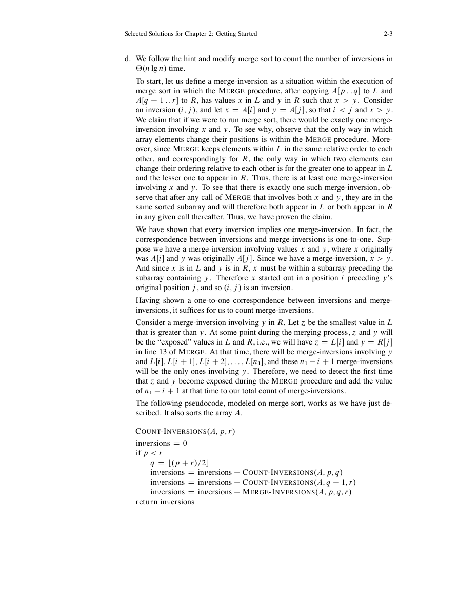The following pseudocode, modeled on merge sort, works as we have just de- scribed. It also sorts the array A. COUNT-INVERSIONS.A; p; r/ inersions D 0 if p < r q D b.p C r/=2c inersions D inersions C COUNT-INVERSIONS.A; p; q/ inersions D inersions C COUNT-INVERSIONS.A; q C 1; r/ inersions D inersions C MERGE-INVERSIONS.A; p; q; r/ return inersions

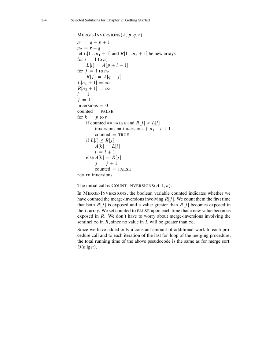
2-4 Selected Solutions for Chapter 2: Getting Started MERGE-INVERSIONS.A; p; q; r/ n1 D q p C 1 n2 D r q let LŒ1 : : n1 C 1 and RŒ1 : : n2 C 1 be new arrays for i D 1 to n1 LŒi D AŒp C i 1 for j D 1 to n2 RŒj D AŒq C j LŒn1 C 1 D 1 RŒn2 C 1 D 1 i D 1 j D 1 inersions D 0 counted D FALSE for k D p to r if counted == FALSE and RŒj < LŒi inersions D inersions C n1 i C 1 counted D TRUE if LŒi RŒj AŒk D LŒi i D i C 1 else AŒk D RŒj j D j C 1 counted D FALSE return inersions The initial call is COUNT-INVERSIONS.A; 1; n/. In MERGE-INVERSIONS, the boolean variable counted indicates whether we have counted the merge-inversions involving RŒj . We count them the ﬁrst time that both RŒj is exposed and a value greater than RŒj becomes exposed in the L array. We set counted to FALSE upon each time that a new value becomes exposed in R. We don’t have to worry about merge-inversions involving the sentinel 1 in R, since no value in L will be greater than 1. Since we have added only a constant amount of additional work to each pro- cedure call and to each iteration of the last for loop of the merging procedure, the total running time of the above pseudocode is the same as for merge sort: ‚.n lg n/.

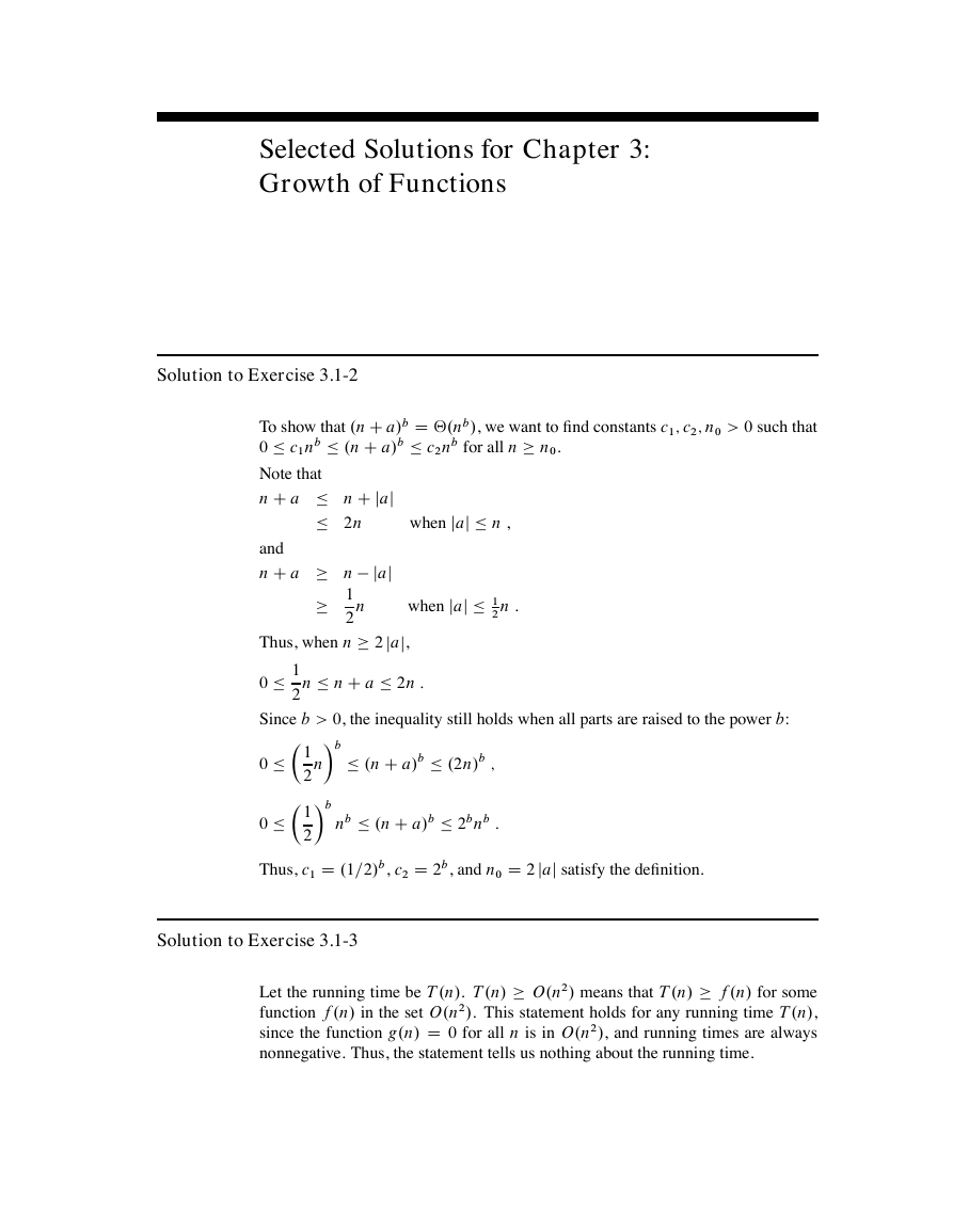
Selected Solutions for Chapter 3: Growth of Functions Solution to Exercise 3.1-2 To show that .n C a/b D ‚.nb/, we want to ﬁnd constants c1; c2; n0 > 0 such that 0 c1nb .n C a/b c2nb for all n n0. Note that n C a n C jaj 2n when jaj n , and n C a n jaj 1 2 n when jaj 1 2 n . Thus, when n 2 jaj, 0 1 2 n n C a 2n : Since b > 0, the inequality still holds when all parts are raised to the power b: 0 b n 1 2 .n C a/b .2n/b ; b 0 1 2 nb .n C a/b 2bnb : Thus, c1 D .1=2/b, c2 D 2b, and n0 D 2 jaj satisfy the deﬁnition. Solution to Exercise 3.1-3 Let the running time be T .n/. T .n/ O.n2/ means that T .n/ f .n/ for some function f .n/ in the set O.n2/. This statement holds for any running time T .n/, since the function g.n/ D 0 for all n is in O.n2/, and running times are always nonnegative. Thus, the statement tells us nothing about the running time.

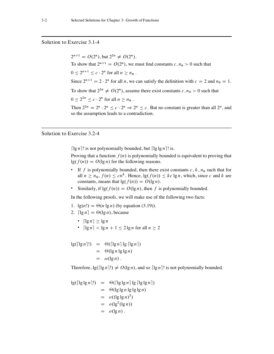
3-2 Selected Solutions for Chapter 3: Growth of Functions Solution to Exercise 3.1-4 2nC1 D O.2n/, but 22n ¤ O.2n/. To show that 2nC1 D O.2n/, we must ﬁnd constants c; n0 > 0 such that 0 2nC1 c 2n for all n n0 : Since 2nC1 D 2 2n for all n, we can satisfy the deﬁnition with c D 2 and n0 D 1. To show that 22n 6D O.2n/, assume there exist constants c; n0 > 0 such that 0 22n c 2n for all n n0 : Then 22n D 2n 2n c 2n ) 2n c. But no constant is greater than all 2n, and so the assumption leads to a contradiction. Solution to Exercise 3.2-4 dlg neŠ is not polynomially bounded, but dlg lg neŠ is. Proving that a function f .n/ is polynomially bounded is equivalent to proving that lg.f .n// D O.lg n/ for the following reasons. If f is polynomially bounded, then there exist constants c, k, n0 such that for all n n0, f .n/ cnk. Hence, lg.f .n// kc lg n, which, since c and k are constants, means that lg.f .n// D O.lg n/. Similarly, if lg.f .n// D O.lg n/, then f is polynomially bounded. In the following proofs, we will make use of the following two facts: lg.nŠ/ D ‚.n lg n/ (by equation (3.19)). 1. 2. dlg ne D ‚.lg n/, because dlg ne lg n dlg ne < lg n C 1 2 lg n for all n 2 lg.dlg neŠ/ D ‚.dlg ne lg dlg ne/ D ‚.lg n lg lg n/ D !.lg n/ : Therefore, lg.dlg neŠ/ ¤ O.lg n/, and so dlg neŠ is not polynomially bounded. lg.dlg lg neŠ/ D ‚.dlg lg ne lg dlg lg ne/ D ‚.lg lg n lg lg lg n/ D o..lg lg n/2/ D o.lg2.lg n// D o.lg n/ :

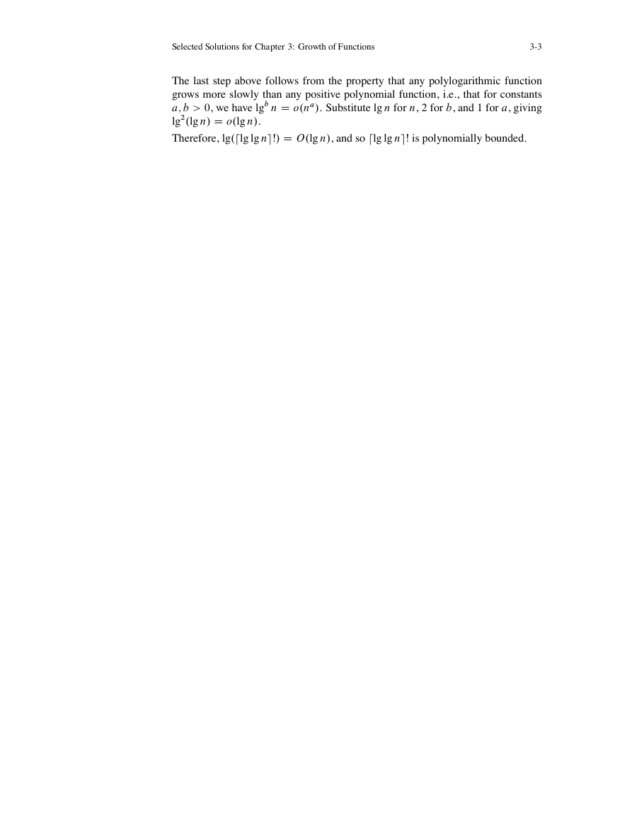
Selected Solutions for Chapter 3: Growth of Functions 3-3 The last step above follows from the property that any polylogarithmic function grows more slowly than any positive polynomial function, i.e., that for constants a; b > 0, we have lgb n D o.na/. Substitute lg n for n, 2 for b, and 1 for a, giving lg2.lg n/ D o.lg n/. Therefore, lg.dlg lg neŠ/ D O.lg n/, and so dlg lg neŠ is polynomially bounded.

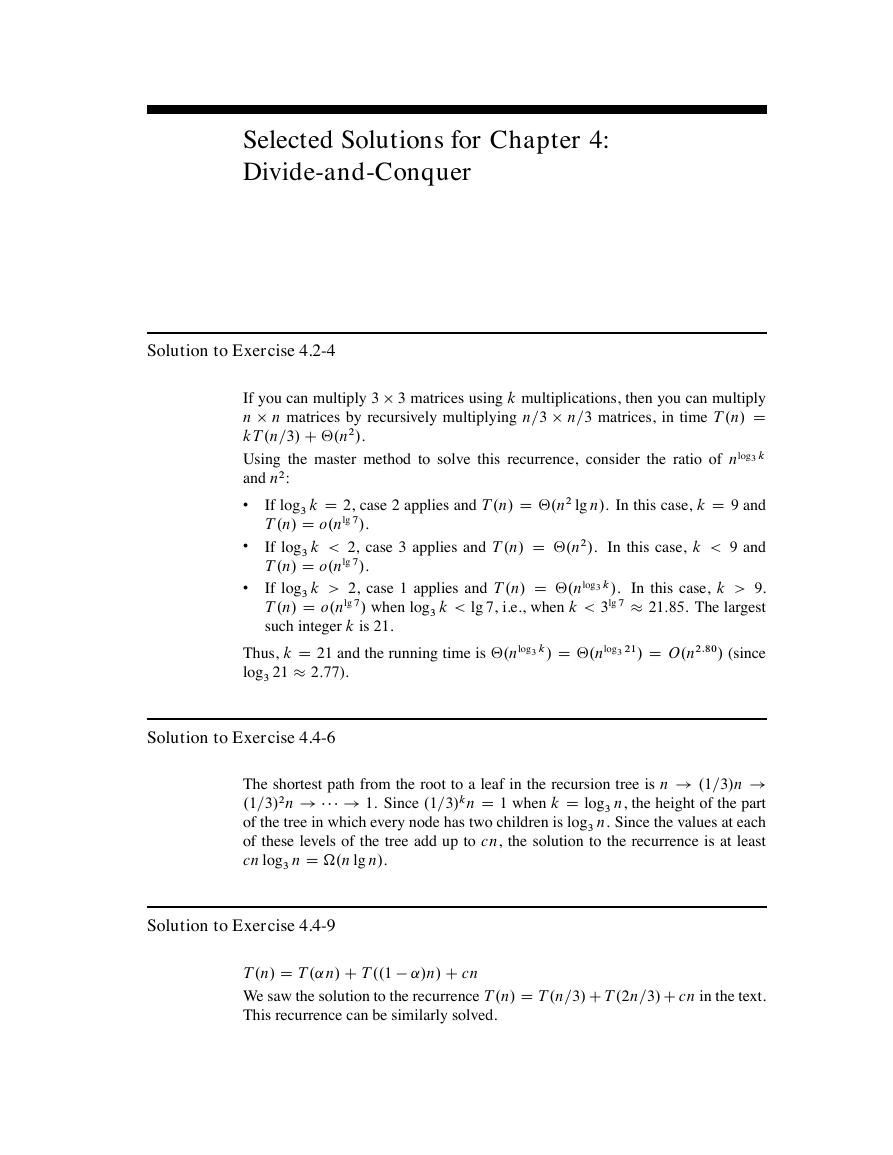
Selected Solutions for Chapter 4: Divide-and-Conquer Solution to Exercise 4.2-4 If you can multiply 3 3 matrices using k multiplications, then you can multiply n n matrices by recursively multiplying n=3 n=3 matrices, in time T .n/ D kT .n=3/ C ‚.n2/. Using the master method to solve this recurrence, consider the ratio of nlog3 k and n2: If log3 k D 2, case 2 applies and T .n/ D ‚.n2 lg n/. In this case, k D 9 and T .n/ D o.nlg 7/. If log3 k < 2, case 3 applies and T .n/ D ‚.n2/. In this case, k < 9 and T .n/ D o.nlg 7/. If log3 k > 2, case 1 applies and T .n/ D ‚.nlog3 k/. In this case, k > 9. T .n/ D o.nlg 7/ when log3 k < lg 7, i.e., when k < 3lg 7 21:85. The largest such integer k is 21. Thus, k D 21 and the running time is ‚.nlog3 k/ D ‚.nlog3 21/ D O.n2:80/ (since log3 21 2:77). Solution to Exercise 4.4-6 The shortest path from the root to a leaf in the recursion tree is n ! .1=3/n ! .1=3/2n ! ! 1. Since .1=3/kn D 1 when k D log3 n, the height of the part of the tree in which every node has two children is log3 n. Since the values at each of these levels of the tree add up to cn, the solution to the recurrence is at least cn log3 n D .n lg n/. Solution to Exercise 4.4-9 T .n/ D T .˛ n/ C T ..1 ˛/n/ C cn We saw the solution to the recurrence T .n/ D T .n=3/ C T .2n=3/ C cn in the text. This recurrence can be similarly solved.

资料库

算法导论第三版答案英文版.pdf

相关推荐

课程资源

热门标签

最新资料