Journal of Geographic Information System, 2019, 11, 196-211
http://www.scirp.org/journal/jgis
ISSN Online: 2151-1969
ISSN Print: 2151-1950
Spatial Modelling of Current and Future Piped
Domestic Water Demand in Athi River Town,
Kenya
Winfred Mbinya Manetu*, Felix Mutua, Benson Kipkemboi Kenduiywo
Department of Geomatic Engineering and Geospatial Information System, Jomo Kenyatta University of Agriculture and
Technology, Nairobi, Kenya
How to cite this paper: Manetu, W.M.,
Mutua, F. and Kenduiywo, B.K. (2019)
Spatial Modelling of Current and Future
Piped Domestic Water Demand in Athi
River Town, Kenya. Journal of Geographic
Information System, 11, 196-211.
https://doi.org/10.4236/jgis.2019.112014
Received: April 9, 2019
Accepted: April 22, 2019
Published: April 25, 2019
Copyright © 2019 by author(s) and
Scientific Research Publishing Inc.
This work is licensed under the Creative
Commons Attribution International
License (CC BY 4.0).
http://creativecommons.org/licenses/by/4.0/
Open Access
Abstract
Water scarcity is currently still a global challenge despite the fact that water
sustains life on earth. An understanding of domestic water demand is there-
fore vital for effective water management. In order to understand and predict
future water demand, appropriate mathematical models are needed. The
present work used Geographic Information Systems (GIS) based regression
models; Geographically weighted regression (GWR) and Ordinary Least
Square (OLS) to model domestic water demand in Athi river town. We iden-
tified a total of 7 water determinant factors in our study area. From these fac-
tors, 4 most significant ones (household size, household income, meter con-
nections and household rooms) were identified using OLS. Further, GWR
technique was used to investigate any intrinsic relationship between the fac-
tors and water demand occurrence. GWR coefficients values computed were
mapped to exhibit the relationship and strength of each explanatory variable
to water demand. By comparing OLS and GWR models with both AIC value
and R2 value, the results demonstrated GWR model as capable of projecting
water demand compared to OLS model. The GWR model was therefore
adopted to predict water demand in the year 2022. It revealed domestic water
demand in 2017 was estimated at 721,899 m3 compared to 880,769 m3 in
2022, explaining an increase of about 22%. Generally, the results of this study
can be used by water resource planners and managers to effectively manage
existing water resources and as baseline information for planning a
cost-effective and reliable water supply sources to the residents of a town.
Keywords
Geographically Weighted Regression, Ordinary Least Square, Water Demand
DOI: 10.4236/jgis.2019.112014 Apr. 25, 2019
196
Journal of Geographic Information System
�
W. M. Manetu et al.
1. Introduction
Water is one of the most important natural goods for maintenance of life in
Earth. Nonetheless, water scarcity is a global challenge that currently affects
more than 40% of the total global population [1]. It is also estimated that by
2025, an estimated 3.9 billion (or over 60%) of the world’s population will live in
a water stressed environment [2]. However, supply of clean and fresh water is
one of the main challenges facing most of the African countries.
Despite water being one of the most essential resources with great implica-
tions for development in Africa, the freshwater situation is still not encouraging
[3]. According to United Nations [4], an estimation of more than 300 million
people in Africa is currently living in a water-scarce environment and many wa-
ter requirements for agriculture, sanitation, industry and domestic use in Africa
cannot be met. Regrettably, the situation is even getting worse as a result of in-
creased population growth, rapid urbanization and industrialization, increasing
agriculture and also lack of adequate capacity to manage existing freshwater re-
sources.
Moreover, in Kenya water predicament remains very critical and the country
has been classified among the water scarce countries with only 647 m3 per capita
against 1000 m3 standard global benchmark [4]. Almost 41% of Kenyans out of a
total population of 46 million people still rely on unimproved water sources,
such as rivers, shallow wells and ponds while 59% of Kenyans use unimproved
sanitation solutions (Kenya water and sanitation report, [5]). Athi River is one of
the Kenya’s fastest growing towns. According to the republic of Kenya 2009
census data, the town’s population growth rate is 4% per annum and it is still
witnessing tremendous growth and social upheaval due to a large influx of new
residents and establishment of new industries. Athi River environment has
therefore been seriously threatened by these alarming population pressures and
industrial development leading to increased water demand [6].
Mavoko Water and Sewerage Company (MAVWASO) owned by the Kenyan
Government, provides sewerage and water services in Athi River town. The
company supplies approximately 3500 m3 of water to a population of around
110,396 per day translating to 40% of the water demand and due to this the area
has frequent water shortage. As a consequence, in order to ensure reliable water
supply to the residents of a town, water demand estimation and projection are
necessary. According to House-Peters et al. [7], water demand estimate is useful
in developing alternative water supply sources, integrating water demand man-
agement programs and also planning a cost effective and reliable infrastructure.
There has been a growing interest in using Geospatial Information System
(GIS) based techniques in modeling water demand occurrence in the recent past
years. According to various studies [8] [9] [10] [11], the interest has mostly
stemmed on analyzing socioeconomic, climate, physical, public policies and
strategies related factors in understanding water demand of a site specific area.
However, water demand modeling can use as many variables as required that
197
Journal of Geographic Information System
DOI: 10.4236/jgis.2019.112014
�
W. M. Manetu et al.
DOI: 10.4236/jgis.2019.112014
directly or indirectly affect the water demand in a particular area. Besides, sever-
al studies have revealed the significance of using ordinary least square (OLS)
technique in identifying key water demand drivers [12] [13]. In a study in Ore-
gon, USA, GIS and statistical methods were used to identify the determinants of
water demand and to determine the water spatial trends and how they changed
overtime [10]. Following the same line, in a study by Wentz et al. [12] that
tackled residential water demand at the census tract level found a spatial effect
above and beyond the effects for household size and pools on water consump-
tion. The results demonstrated that census tracts exhibited water consumption
behavior similar to neighboring tracts for the two variables. However, occur-
rence of critical water shortage issues reported in Athi River town has been
highly associated with socioeconomic characteristics which indicate the eco-
nomic status of the region [6]. Modeling them can help understand the key fac-
tors in terms of their influence, pattern and relationship they have to water use.
With the rise of new statistical techniques and GIS tools, GIS techniques have
come in handy in analyzing and estimating water use/demand. In spite of this,
research on water demand occurrence in Kenya has been done but most studies
like [14] [15] [16] [17] [18] have not yet utilized GIS spatial modeling techniques
to its full potential. Narrowing down to the study’s area of interest, despite the
town having frequent water shortages, few studies [19] [20] has been conducted
to analyze the problematic situation of the town and none of the studies have
incorporated the idea of GIS technology to understand this water use challenge
in a spatial domain. GIS is a new technique which has been recently used to
analyze and understand the factors behind water demand and to estimate its oc-
currence for sometimes in future.
Therefore, this study explored the use of GIS spatial modeling to examine the
effects of housing characteristics on water use at the zone level in Athi River
town. This was arrived at, first of all by determining factors that influence do-
mestic water demand occurrence in the town. We achieved this by applying a
global OLS regression model to select the significant factors from candidate fac-
tors proposed to use when assessing domestic water demand. Secondly, local
GWR regression model was adopted in orderto reveal the sensitivity selected
factors to water use and examine their spatial effects above and beyond domestic
water use. Finally, the study used the GWR model to project short term water
use of the town. This baseline information can be useful in administering and
planning adequate water supply system.
2. Materials and Methods
2.1. Study Area
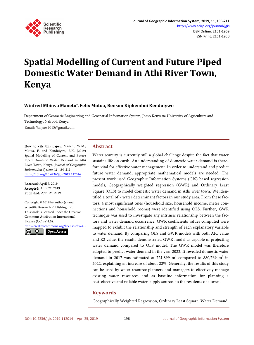
Athi River town was targeted for the analysis because of its heterogeneous cha-
racteristics. For instance; Senior staff is an area with very low population and
well supplied with piped water, Ngei 2 represents a middle class area, Sofia and
slota are slum areas with high population and less piped water connection, and
198
Journal of Geographic Information System
�
W. M. Manetu et al.
Old town is a commercial centre. To enhance water service delivery, the town is
divided into thirty-nine subzones regions (Figure 1).
2.2. Description of Data
The data collected in order to achieve the objectives of this study included
both primary, and secondary data. Primary data were collected through the use
of close and open-ended questionnaires, interviews and field observations.
Face-to-face interviews were administered with the senior and junior staffs at
MAVWASCO. Observations were made through several visits to the sites whe-
reas questionnaires were administered to the residents of the town. This enabled
us to have firsthand information on key household characteristics which were
hypothesized as key independent variables that influence water consumption in
our study area. The variables included data on average household rooms, per-
centage of people with diploma holder and above (education level), average
household income and the percentage of households with garden. GIS vector
data in shape file format of the meter connection was obtained from the GIS
Department of MAVWASCO. Population data was obtained from the Kenya
GIS Portal as provided by the Kenya National Bureau of Statistics per national
2009 census count. The population data had lot of metadata such as age and
gender which was not required in the analysis hence these columns were deleted.
A geodatabase of the domestic water demand for the area was created using
ArcGIS 10.2 and the information captured included; average household size,
number of meter connections, number of households, average household rooms,
average household income, percentage of households with garden presence and
percentage of people with diploma holder and above (education level). The geo-
database formed the platform on which various analysis were done. Administra-
tive datasets for Mavoko sub-county were obtained from the Machakos County
Government. The dataset was used to delineate Athi River township boundary.
The shape file generated outlined the boundaries of all the 39 zones which get
water supply from the company. For the dependent variable, we used 2017 bill-
ing records for water consumption to determine factors affecting the total con-
sumption of residential units at the zone level in Athi River Town. Water con-
sumption data for all sectors were acquired from Mavoko Water and Sewerage
Company, Commercial Department. We extracted only domestic water users
from their database, combined the monthly data for the year 2017, and aggre-
gated use to the zone level in order to protect the privacy of individual house-
holds. These statistical values were entered into the prepared GIS vector polygon
map as non-spatial data. Lastly, all the data were converted to ESRI Shape files
and transformed to one coordinate system Universal Transverse Mercator
(UTM) zone 37-S on WGS_1984 datum and file geodatabase which was used for
the analysis was created in arc catalogue in ArcGIS where all feature classes were
created and stored considering the compatibility of the dataset in terms of for-
mats, scale and types.
199
Journal of Geographic Information System
DOI: 10.4236/jgis.2019.112014
�
W. M. Manetu et al.
Figure 1. Map of the study area.
2.3. Methods
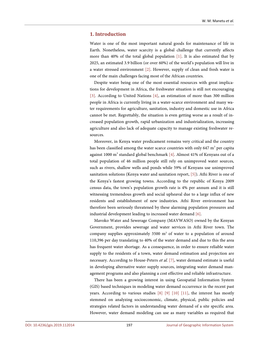
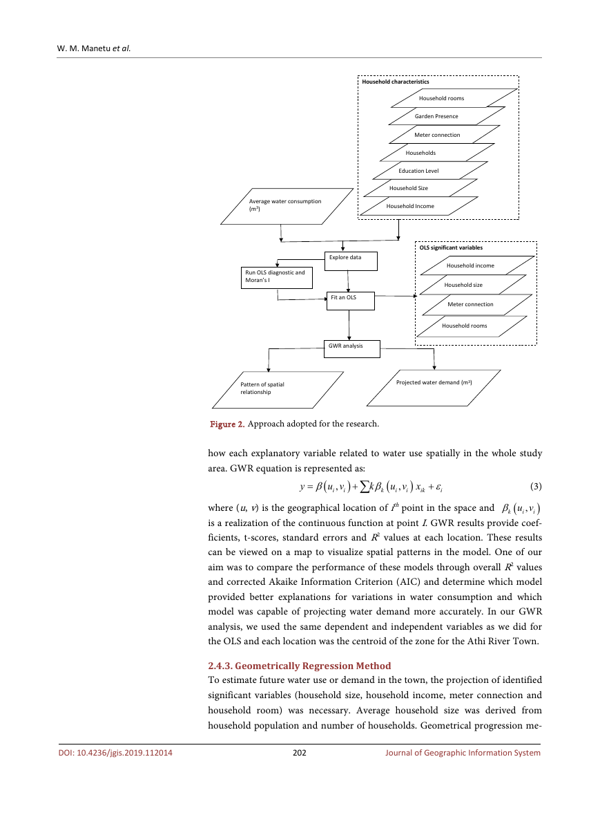
We adopted the approach as shown in Figure 2 in order to examine the effects of
housing characteristics on water use at the zone level in Athi River town. To begin
with, household characteristics that are proposed to use in assessing water demand
were determined from various studies and used as the independent variables in
this study. Consequently, using the identified household characteristics as the ex-
planatory variables and recorded water consumption for 2017 by zone level as
the dependent variable, Ordinary Least Squares (OLS) and Geographically
Weighted Regression (GWR) models were applied to understand domestic
water demand in Athi river. OLS regression model was used to check for multi-
collinearity effects among the explanatory variables and for selecting the signifi-
cant variables. In addition, spatial autocorrelation statistic was applied to detect
whether there was spatial autocorrelation or clustering of the residuals which vi-
olate the assumptions of OLS. Finally, in order to examine the spatial relation-
ship between the significant variables and water demand occurrence and in pre-
dicting future water demand of the town, GWR regression model was adopted.
2.4. Analysis Methods
2.4.1. Ordinary Least Square Regression
Several factors from literature have been proposed for use in assessing water
demand/use occurrence in site-specific area. For instance, these studies [6]-[11],
[17] established use of around 10 household characteristics to have influence in
domestic water use. They included; household size, household income, educa-
tion level, building age, number of rooms, garden, swimming pool, lot size, me-
ter connection and number of households. From field visits and talk to munici-
pal senior and junior staffs and residents, only 7 of the 10 variables were found
200
Journal of Geographic Information System
DOI: 10.4236/jgis.2019.112014
�
W. M. Manetu et al.
relevant to our study area (Figure 2). In order to narrow down and determine
the significant variables, the above mentioned 10 factors were considered and
subjected to OLS regression against a dependent variable to determine its signi-
ficance in the study. OLS is commonly referred to as linear regression because of
the nature of its model. The model can be simple or multiple depending on the
number of explanatory variables. The OLS method corresponds to minimizing
the sum of square differences between the observed and predicted values. As
long as a model satisfies the assumptions of the OLS for linear regression, then
the best possible estimates can be guaranteed. The study therefore used OLS
technique for selecting the appropriate key predictors of domestic water demand
with respect to their type and strength of relationship with the dependent varia-
ble. The OLS models equation can be expressed as:
x
+
n n
(1)
β ε
x
2 2
x
3 3
x
1 1
y
=
β β β β
+
+
+
0
where y is the dependent variable, beta β represents the contribution of each in-
dependent variable makes to the prediction of dependent variable, x is the cor-
responding number of predictors and ε is the random error term of the resi-
duals. In our study, water consumption was the dependent variable with average
household size, average household income, education level, building age, num-
ber of rooms, garden, meter connection and number of households as the inde-
pendent variables. Essentially, OLS model was also used to check for multicolli-
nearity effects (redundancy among predictors). The multicollinearity was as-
sessed with the variance inflation factor (VIF) values of the OLS. As proposed by
[21], the VIF of the ith predictor can be expressed by;
VIF
=
1
2
R i
−
1
(2)
where R2 is the multiple correlation coefficients of the regression and i is the
predictors. If the computed VIF value(s) is greater than 7.5, it indicates the ex-
istence of multicollinearity among the predictors. Progressively, spatial auto-
correlation statistic was applied to detect whether there was clustering of the resi-
duals which violates the assumption of OLS. As well, the spatial independency of
the residuals was assessed with the global spatial autocorrelation coefficient (Mo-
ran’s I).
2.4.2. Geographically Weighted Regression
GWR is a tool for exploring spatial heterogeneity; it allows the relationships be-
ing modelled to vary across the study area. The GWR is designed to answer
scientific questions like, which explanatory variable shows stronger influence in
a certain area? Does the relationship between the dependent variable and the
predictors vary across space? Our expectation is that the variation in water de-
mand is a function of both the effects of the independent variables on domestic
water demand and the fact that the nearby zones are similar with respect to the
independent variables. Therefore, the GWR was adopted in the study to explore
201
Journal of Geographic Information System
DOI: 10.4236/jgis.2019.112014
�
W. M. Manetu et al.
Household characteristics
Household rooms
Garden Presence
Meter connection
Households
Education Level
Household Size
Household Income
OLS significant variables
Household income
Household size
Meter connection
Household rooms
Explore data
Fit an OLS
GWR analysis
Average water consumption
(m3)
Run OLS diagnostic and
Moran’s I
Pattern of spatial
relationship
Projected water demand (m3)
y
=
)
(
)
x
ik
β
k
(
(
β
+
ε
i
u v
,
i
i
u v
,
i
i
Figure 2. Approach adopted for the research.
how each explanatory variable related to water use spatially in the whole study
area. GWR equation is represented as:
+ ∑
k
(3)
)
where (u, v) is the geographical location of ith point in the space and
is a realization of the continuous function at point I. GWR results provide coef-
ficients, t-scores, standard errors and R2 values at each location. These results
can be viewed on a map to visualize spatial patterns in the model. One of our
aim was to compare the performance of these models through overall R2 values
and corrected Akaike Information Criterion (AIC) and determine which model
provided better explanations for variations in water consumption and which
model was capable of projecting water demand more accurately. In our GWR
analysis, we used the same dependent and independent variables as we did for
the OLS and each location was the centroid of the zone for the Athi River Town.
u vβ
,
i
k
i
2.4.3. Geometrically Regression Method
To estimate future water use or demand in the town, the projection of identified
significant variables (household size, household income, meter connection and
household room) was necessary. Average household size was derived from
household population and number of households. Geometrical progression me-
202
Journal of Geographic Information System
DOI: 10.4236/jgis.2019.112014
�
W. M. Manetu et al.
thod was used in estimating population (in this method the percentage increase
in population from year to year was assumed to remain constant at 4% per an-
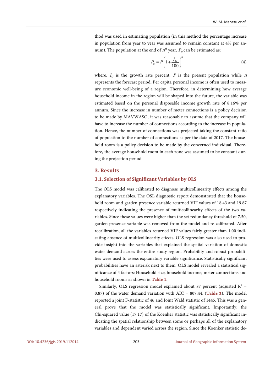
num). The population at the end of nth year, Pn can be estimated as:
P
n
=
n
P
1
+
I
G
100
(4)
where, IG is the growth rate percent, P is the present population while n
represents the forecast period. Per capita personal income is often used to meas-
ure economic well-being of a region. Therefore, in determining how average
household income in the region will be shaped into the future, the variable was
estimated based on the personal disposable income growth rate of 8.16% per
annum. Since the increase in number of meter connections is a policy decision
to be made by MAVWASO, it was reasonable to assume that the company will
have to increase the number of connections according to the increase in popula-
tion. Hence, the number of connections was projected taking the constant ratio
of population to the number of connections as per the data of 2017. The house-
hold room is a policy decision to be made by the concerned individual. There-
fore, the average household room in each zone was assumed to be constant dur-
ing the projection period.
3. Results
3.1. Selection of Significant Variables by OLS
The OLS model was calibrated to diagnose multicollinearity effects among the
explanatory variables. The OSL diagnostic report demonstrated that the house-
hold room and garden presence variable returned VIF values of 18.43 and 19.87
respectively indicating the presence of multicollinearity effects of the two va-
riables. Since these values were higher than the set redundancy threshold of 7.50,
garden presence variable was removed from the model and re-calibrated. After
recalibration, all the variables returned VIF values fairly greater than 1.00 indi-
cating absence of multicollinearity effects. OLS regression was also used to pro-
vide insight into the variables that explained the spatial variation of domestic
water demand across the entire study region. Probability and robust probabili-
ties were used to assess explanatory variable significance. Statistically significant
probabilities have an asterisk next to them. OLS model revealed a statistical sig-
nificance of 4 factors: Household size, household income, meter connections and
household rooms as shown in Table 1.
Similarly, OLS regression model explained about 87 percent (adjusted R2 =
0.87) of the water demand variation with AIC = 807.44, (Table 2). The model
reported a joint F-statistic of 46 and Joint Wald statistic of 1445. This was a gen-
eral prove that the model was statistically significant. Importantly, the
Chi-squared value (17.17) of the Koenker statistic was statistically significant in-
dicating the spatial relationship between some or perhaps all of the explanatory
variables and dependent varied across the region. Since the Koenker statistic de-
203
Journal of Geographic Information System
DOI: 10.4236/jgis.2019.112014
�




 2023年江西萍乡中考道德与法治真题及答案.doc
 2012年重庆南川中考生物真题及答案.doc
 2013年江西师范大学地理学综合及文艺理论基础考研真题.doc
 2020年四川甘孜小升初语文真题及答案I卷.doc
 2020年注册岩土工程师专业基础考试真题及答案.doc
 2023-2024学年福建省厦门市九年级上学期数学月考试题及答案.doc
 2021-2022学年辽宁省沈阳市大东区九年级上学期语文期末试题及答案.doc
 2022-2023学年北京东城区初三第一学期物理期末试卷及答案.doc
 2018上半年江西教师资格初中地理学科知识与教学能力真题及答案.doc
 2012年河北国家公务员申论考试真题及答案-省级.doc
 2020-2021学年江苏省扬州市江都区邵樊片九年级上学期数学第一次质量检测试题及答案.doc
 2022下半年黑龙江教师资格证中学综合素质真题及答案.doc