Y. Liu et al. / Information Fusion 36 (2017) 191–207
193
activation [41] applied in CNNs are jointly expressed as
j =
y
i j ∗ x
i )
k
j +
b
max
(0
,
,
i
full connection operation can be viewed as convolution with the
kernel size that equals to the spatial size of input data [45] ), it is
practically feasible to apply CNNs to image fusion.
(1)
}
,
n
∗
(2)
i
y
r,c
i
r·s
+
x
m,c·s
+
× d
i and y
ij is the convolutional kernel between x
j
j , and b
where k
indicates convolutional operation. When
is the bias. The symbol
there are M input maps and N output maps, this layer will contain
× M ( d
× d is the size of local recep-
N 3D kernels of size d
tive fields) and each kernel owns a bias. The last idea sub-sampling
is also known as pooling, which can reduce data dimension. Max-
pooling and average-pooling are popular operations in CNNs. As an
example, the max-pooling operation is formulated as
× s in the i -th input map x
{
=
max
≤m,n
194
Y. Liu et al. / Information Fusion 36 (2017) 191–207
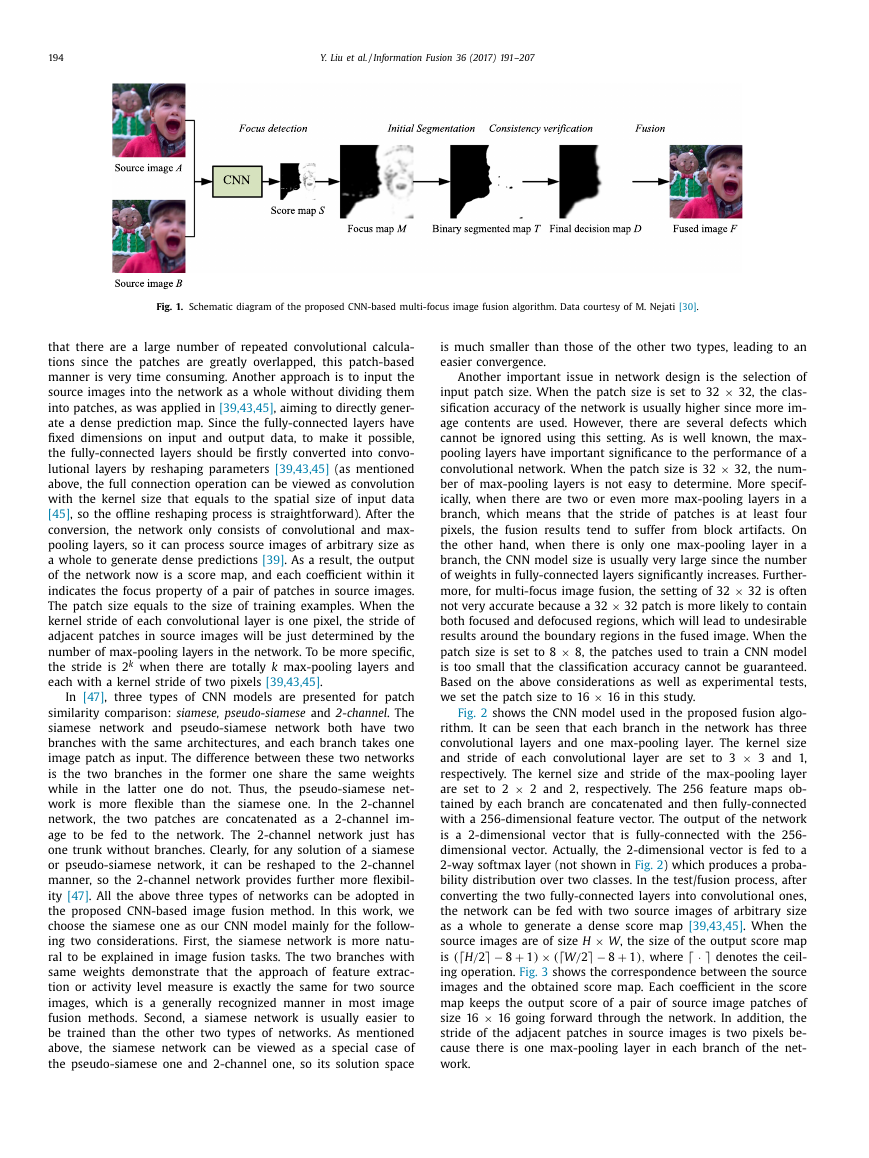
Fig. 1. Schematic diagram of the proposed CNN-based multi-focus image fusion algorithm. Data courtesy of M. Nejati [30] .
that there are a large number of repeated convolutional calcula-
tions since the patches are greatly overlapped, this patch-based
manner is very time consuming. Another approach is to input the
source images into the network as a whole without dividing them
into patches, as was applied in [39,43,45] , aiming to directly gener-
ate a dense prediction map. Since the fully-connected layers have
fixed dimensions on input and output data, to make it possible,
the fully-connected layers should be firstly converted into convo-
lutional layers by reshaping parameters [39,43,45] (as mentioned
above, the full connection operation can be viewed as convolution
with the kernel size that equals to the spatial size of input data
[45] , so the offline reshaping process is straightforward). After the
conversion, the network only consists of convolutional and max-
pooling layers, so it can process source images of arbitrary size as
a whole to generate dense predictions [39] . As a result, the output
of the network now is a score map, and each coefficient within it
indicates the focus property of a pair of patches in source images.
The patch size equals to the size of training examples. When the
kernel stride of each convolutional layer is one pixel, the stride of
adjacent patches in source images will be just determined by the
number of max-pooling layers in the network. To be more specific,
k when there are totally k max-pooling layers and
the stride is 2
each with a kernel stride of two pixels [39,43,45] .
In [47] , three types of CNN models are presented for patch
similarity comparison: siamese, pseudo-siamese and 2-channel . The
siamese network and pseudo-siamese network both have two
branches with the same architectures, and each branch takes one
image patch as input. The difference between these two networks
is the two branches in the former one share the same weights
while in the latter one do not. Thus, the pseudo-siamese net-
work is more flexible than the siamese one. In the 2-channel
network, the two patches are concatenated as a 2-channel im-
age to be fed to the network. The 2-channel network just has
one trunk without branches. Clearly, for any solution of a siamese
or pseudo-siamese network, it can be reshaped to the 2-channel
manner, so the 2-channel network provides further more flexibil-
ity [47] . All the above three types of networks can be adopted in
the proposed CNN-based image fusion method. In this work, we
choose the siamese one as our CNN model mainly for the follow-
ing two considerations. First, the siamese network is more natu-
ral to be explained in image fusion tasks. The two branches with
same weights demonstrate that the approach of feature extrac-
tion or activity level measure is exactly the same for two source
images, which is a generally recognized manner in most image
fusion methods. Second, a siamese network is usually easier to
be trained than the other two types of networks. As mentioned
above, the siamese network can be viewed as a special case of
the pseudo-siamese one and 2-channel one, so its solution space
is much smaller than those of the other two types, leading to an
easier convergence.
Another important issue in network design is the selection of
× 32, the clas-
input patch size. When the patch size is set to 32
sification accuracy of the network is usually higher since more im-
age contents are used. However, there are several defects which
cannot be ignored using this setting. As is well known, the max-
pooling layers have important significance to the performance of a
× 32, the num-
convolutional network. When the patch size is 32
ber of max-pooling layers is not easy to determine. More specif-
ically, when there are two or even more max-pooling layers in a
branch, which means that the stride of patches is at least four
pixels, the fusion results tend to suffer from block artifacts. On
the other hand, when there is only one max-pooling layer in a
branch, the CNN model size is usually very large since the number
of weights in fully-connected layers significantly increases. Further-
× 32 is often
more, for multi-focus image fusion, the setting of 32
× 32 patch is more likely to contain
not very accurate because a 32
both focused and defocused regions, which will lead to undesirable
results around the boundary regions in the fused image. When the
× 8, the patches used to train a CNN model
patch size is set to 8
is too small that the classification accuracy cannot be guaranteed.
Based on the above considerations as well as experimental tests,
we set the patch size to 16
× 16 in this study.
Fig. 2 shows the CNN model used in the proposed fusion algo-
rithm. It can be seen that each branch in the network has three
convolutional layers and one max-pooling layer. The kernel size
× 3 and 1,
and stride of each convolutional layer are set to 3
respectively. The kernel size and stride of the max-pooling layer
× 2 and 2, respectively. The 256 feature maps ob-
are set to 2
tained by each branch are concatenated and then fully-connected
with a 256-dimensional feature vector. The output of the network
is a 2-dimensional vector that is fully-connected with the 256-
dimensional vector. Actually, the 2-dimensional vector is fed to a
2-way softmax layer (not shown in Fig. 2 ) which produces a proba-
bility distribution over two classes. In the test/fusion process, after
converting the two fully-connected layers into convolutional ones,
the network can be fed with two source images of arbitrary size
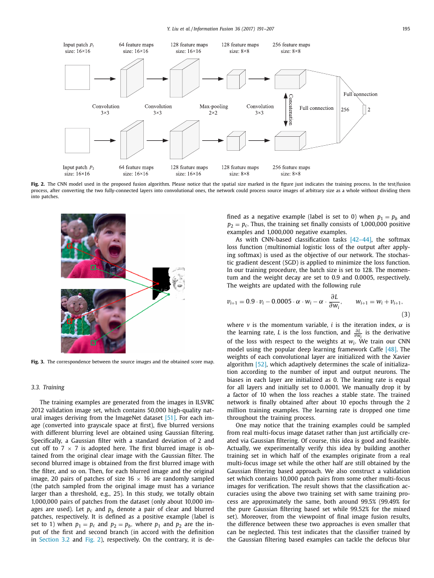
as a whole to generate a dense score map [39,43,45] . When the
× W , the size of the output score map
source images are of size H
− 8
+
(
is
denotes the ceil-
ing operation. Fig. 3 shows the correspondence between the source
images and the obtained score map. Each coefficient in the score
map keeps the output score of a pair of source image patches of
× 16 going forward through the network. In addition, the
size 16
stride of the adjacent patches in source images is two pixels be-
cause there is one max-pooling layer in each branch of the net-
work.
− 8
+
,
where
W/
2
·
× (
1)
2
H/
1)
�
Y. Liu et al. / Information Fusion 36 (2017) 191–207
195
Fig. 2. The CNN model used in the proposed fusion algorithm. Please notice that the spatial size marked in the figure just indicates the training process. In the test/fusion
process, after converting the two fully-connected layers into convolutional ones, the network could process source images of arbitrary size as a whole without dividing them
into patches.
=
fined as a negative example (label is set to 0) when p 1
=
p 2
examples and 1,0 0 0,0 0 0 negative examples.
and
p c . Thus, the training set finally consists of 1,0 0 0,0 0 0 positive
p b
As with CNN-based classification tasks [42–44] , the softmax
loss function (multinomial logistic loss of the output after apply-
ing softmax) is used as the objective of our network. The stochas-
tic gradient descent (SGD) is applied to minimize the loss function.
In our training procedure, the batch size is set to 128. The momen-
tum and the weight decay are set to 0.9 and 0.0 0 05, respectively.
The weights are updated with the following rule
=
+1
.
0
9
· v i
v i
− 0
.
0 0 05
· α · w i
− α · ∂L
,
w i
∂
=
+
v i
+1
w i
+1
,
w i
Fig. 3. The correspondence between the source images and the obtained score map.
3.3. Training
The training examples are generated from the images in ILSVRC
2012 validation image set, which contains 50,0 0 0 high-quality nat-
ural images deriving from the ImageNet dataset [51] . For each im-
age (converted into grayscale space at first), five blurred versions
with different blurring level are obtained using Gaussian filtering.
Specifically, a Gaussian filter with a standard deviation of 2 and
× 7 is adopted here. The first blurred image is ob-
cut off to 7
tained from the original clear image with the Gaussian filter. The
second blurred image is obtained from the first blurred image with
the filter, and so on. Then, for each blurred image and the original
× 16 are randomly sampled
image, 20 pairs of patches of size 16
(the patch sampled from the original image must has a variance
larger than a threshold, e.g., 25). In this study, we totally obtain
1,0 0 0,0 0 0 pairs of patches from the dataset (only about 10,0 0 0 im-
denote a pair of clear and blurred
ages are used). Let p c and p b
patches, respectively. It is defined as a positive example (label is
=
=
set to 1) when p 1
are the in-
p c and p 2
put of the first and second branch (in accord with the definition
in Section 3.2 and Fig. 2 ), respectively. On the contrary, it is de-
,
p b
where p 1
and p 2
(3)
α is
is the derivative
where v is the momentum variable, i is the iteration index,
∂L
the learning rate, L is the loss function, and
∂
w i
of the loss with respect to the weights at w i
. We train our CNN
model using the popular deep learning framework Caffe [48] . The
weights of each convolutional layer are initialized with the Xavier
algorithm [52] , which adaptively determines the scale of initializa-
tion according to the number of input and output neurons. The
biases in each layer are initialized as 0. The leaning rate is equal
for all layers and initially set to 0.0 0 01. We manually drop it by
a factor of 10 when the loss reaches a stable state. The trained
network is finally obtained after about 10 epochs through the 2
million training examples. The learning rate is dropped one time
throughout the training process.
One may notice that the training examples could be sampled
from real multi-focus image dataset rather than just artificially cre-
ated via Gaussian filtering. Of course, this idea is good and feasible.
Actually, we experimentally verify this idea by building another
training set in which half of the examples originate from a real
multi-focus image set while the other half are still obtained by the
Gaussian filtering based approach. We also construct a validation
set which contains 10,0 0 0 patch pairs from some other multi-focus
images for verification. The result shows that the classification ac-
curacies using the above two training set with same training pro-
cess are approximately the same, both around 99.5% (99.49% for
the pure Gaussian filtering based set while 99.52% for the mixed
set). Moreover, from the viewpoint of final image fusion results,
the difference between these two approaches is even smaller that
can be neglected. This test indicates that the classifier trained by
the Gaussian filtering based examples can tackle the defocus blur
�
196
Y. Liu et al. / Information Fusion 36 (2017) 191–207
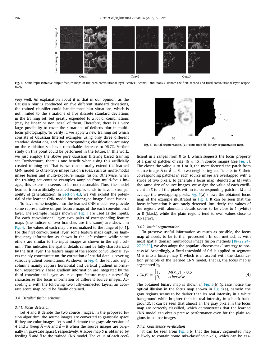
Fig. 4. Some representative output feature maps of the each convolutional layer. “conv1”, “conv2” and “conv3” denote the first, second and third convolutional layer, respec-
tively.
very well. An explanation about it is that in our opinion, as the
Gaussian blur is conducted on five different standard deviations,
the trained classifier could handle most blur situations, which is
not limited to the situations of five discrete standard deviations
in the training set, but greatly expended to a lot of combinations
(may be linear or nonlinear) of them. Therefore, there is a very
large possibility to cover the situations of defocus blur in multi-
focus photography. To verify it, we apply a new training set which
consists of Gaussian filtered examples using only three different
standard deviations, and the corresponding classification accuracy
on the validation set has a remarkable decrease to 96.7%. Further
study on this point could be performed in the future. In this work,
we just employ the above pure Gaussian filtering based training
set. Furthermore, there is one benefit when using this artificially
created training set. That is, we can naturally extend the learned
CNN model to other-type image fusion issues, such as multi-modal
image fusion and multi-exposure image fusion. Otherwise, when
the training set contains examples sampled from multi-focus im-
ages, this extension seems to be not reasonable. Thus, the model
learned from artificially created examples tends to have a stronger
ability of generalization. In Section 4.3 , we will exhibit the poten-
tial of the learned CNN model for other-type image fusion issues.
To have some insights into the learned CNN model, we provide
some representative output feature maps of the each convolutional
layer. The example images shown in Fig. 1 are used as the inputs.
For each convolutional layer, two pairs of corresponding feature
maps (the indices of two branches are the same) are shown in
Fig. 4 . The values of each map are normalized to the range of [0, 1].
For the first convolutional layer, some feature maps captures high-
frequency information as shown in the left column while some
others are similar to the input images as shown in the right col-
umn. This indicates the spatial details cannot be fully characterized
by the first layer. The feature maps of the second convolutional lay-
ers mainly concentrate on the extraction of spatial details covering
various gradient orientations. As shown in Fig. 4 , the left and right
columns mainly capture horizontal and vertical gradient informa-
tion, respectively. These gradient information are integrated by the
third convolutional layer, as its output feature maps successfully
characterize the focus information of different source images. Ac-
cordingly, with the following two fully-connected layers, an accu-
rate score map could be finally obtained.
3.4. Detailed fusion scheme
3.4.1. Focus detection
Let A and B denote the two source images. In the proposed fu-
sion algorithm, the source images are converted to grayscale space
if they are color images. Let ˆ A and ˆ B denote the grayscale version of
=
A and B (keep ˆ A
B when the source images are origi-
nally in grayscale space), respectively. A score map S is obtained by
feeding ˆ A and ˆ B to the trained CNN model. The value of each coef-
=
A and ˆ B
Fig. 5. Initial segmentation. (a) Focus map (b) binary segmentation map.
ficient in S ranges from 0 to 1, which suggests the focus property
× 16 in source images (see Fig. 3 ).
of a pair of patches of size 16
The closer the value is to 1 or 0, the more focused the patch from
source image ˆ A or ˆ B is. For two neighboring coefficients in S , their
corresponding patches in each source image are overlapped with a
stride of two pixels. To generate a focus map (denoted as M ) with
the same size of source images, we assign the value of each coeffi-
cient in S to all the pixels within its corresponding patch in M and
average the overlapping pixels. Fig. 5 (a) shows the obtained focus
map of the example illustrated in Fig. 1 . It can be seen that the
focus information is accurately detected. Intuitively, the values of
the regions with abundant details seems to be close to 1 (white)
or 0 (black), while the plain regions tend to own values close to
0.5 (gray).
3.4.2. Initial segmentation
To preserve useful information as much as possible, the focus
map M needs to be further processed . In our method, as with
most spatial domain multi-focus image fusion methods [18–22,24–
27,29,30] , we also adopt the popular “choose-max” strategy to pro-
cess M . Accordingly, a fixed threshold of 0.5 is applied to segment
M is into a binary map T , which is in accord with the classifica-
tion principle of the learned CNN model. That is, the focus map is
segmented by
,
1
,
0
(x,
T
)
y
=
M(x,
)
y
>
otherwise
.
5
0
.
(4)
The obtained binary map is shown in Fig. 5 (b) (please notice the
optical illusion in the focus map shown in Fig. 5 (a), namely, the
gray regions seems to be darker than its real intensity in a white
background while brighter than its real intensity in a black back-
ground). It can be seen that almost all the gray pixels in the focus
map are correctly classified, which demonstrates that the learned
CNN model can obtain precise performance even for the plain re-
gions in source images.
3.4.3. Consistency verification
It can be seen from Fig. 5 (b) that the binary segmented map
is likely to contain some mis-classified pixels, which can be eas-
�
Y. Liu et al. / Information Fusion 36 (2017) 191–207
197
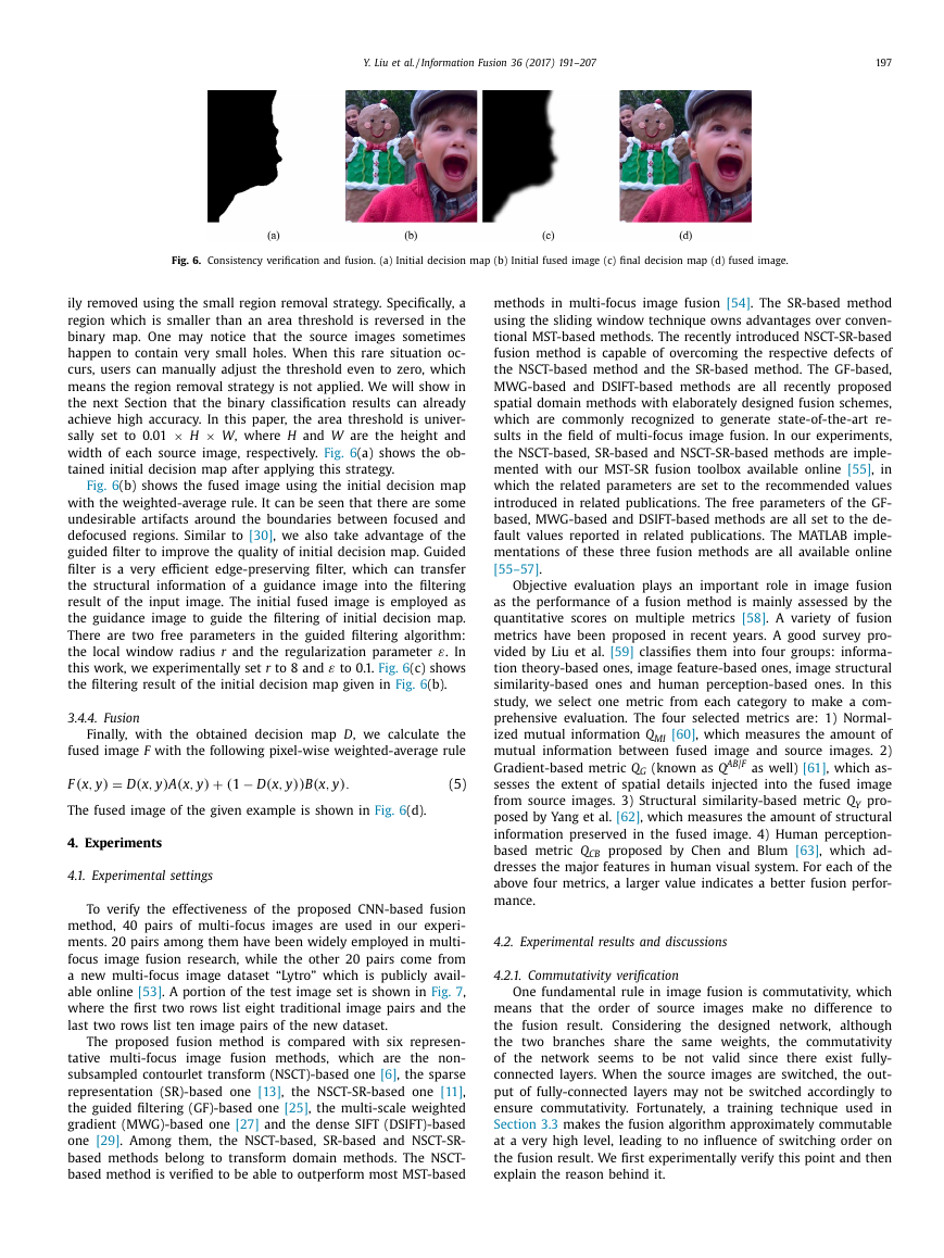
Fig. 6. Consistency verification and fusion. (a) Initial decision map (b) Initial fused image (c) final decision map (d) fused image.
ily removed using the small region removal strategy. Specifically, a
region which is smaller than an area threshold is reversed in the
binary map. One may notice that the source images sometimes
happen to contain very small holes. When this rare situation oc-
curs, users can manually adjust the threshold even to zero, which
means the region removal strategy is not applied. We will show in
the next Section that the binary classification results can already
achieve high accuracy. In this paper, the area threshold is univer-
× W , where H and W are the height and
sally set to 0.01
width of each source image, respectively. Fig. 6 (a) shows the ob-
tained initial decision map after applying this strategy.
× H
Fig. 6 (b) shows the fused image using the initial decision map
with the weighted-average rule. It can be seen that there are some
undesirable artifacts around the boundaries between focused and
defocused regions. Similar to [30] , we also take advantage of the
guided filter to improve the quality of initial decision map. Guided
filter is a very efficient edge-preserving filter, which can transfer
the structural information of a guidance image into the filtering
result of the input image. The initial fused image is employed as
the guidance image to guide the filtering of initial decision map.
There are two free parameters in the guided filtering algorithm:
ε. In
the local window radius r and the regularization parameter
ε to 0.1. Fig. 6 (c) shows
this work, we experimentally set r to 8 and
the filtering result of the initial decision map given in Fig. 6 (b).
3.4.4. Fusion
Finally, with the obtained decision map D , we calculate the
fused image F with the following pixel-wise weighted-average rule
(x,
F
)
y
=
D
(x,
)
y
(x,
A
)
y
+
− D
(x,
(1
))
y
(x,
B
)
y
.
(5)
The fused image of the given example is shown in Fig. 6 (d).
4. Experiments
4.1. Experimental settings
To verify the effectiveness of the proposed CNN-based fusion
method, 40 pairs of multi-focus images are used in our experi-
ments. 20 pairs among them have been widely employed in multi-
focus image fusion research, while the other 20 pairs come from
a new multi-focus image dataset “Lytro” which is publicly avail-
able online [53] . A portion of the test image set is shown in Fig. 7 ,
where the first two rows list eight traditional image pairs and the
last two rows list ten image pairs of the new dataset.
The proposed fusion method is compared with six represen-
tative multi-focus image fusion methods, which are the non-
subsampled contourlet transform (NSCT)-based one [6] , the sparse
representation (SR)-based one [13] , the NSCT-SR-based one [11] ,
the guided filtering (GF)-based one [25] , the multi-scale weighted
gradient (MWG)-based one [27] and the dense SIFT (DSIFT)-based
one [29] . Among them, the NSCT-based, SR-based and NSCT-SR-
based methods belong to transform domain methods. The NSCT-
based method is verified to be able to outperform most MST-based
methods in multi-focus image fusion [54] . The SR-based method
using the sliding window technique owns advantages over conven-
tional MST-based methods. The recently introduced NSCT-SR-based
fusion method is capable of overcoming the respective defects of
the NSCT-based method and the SR-based method. The GF-based,
MWG-based and DSIFT-based methods are all recently proposed
spatial domain methods with elaborately designed fusion schemes,
which are commonly recognized to generate state-of-the-art re-
sults in the field of multi-focus image fusion. In our experiments,
the NSCT-based, SR-based and NSCT-SR-based methods are imple-
mented with our MST-SR fusion toolbox available online [55] , in
which the related parameters are set to the recommended values
introduced in related publications. The free parameters of the GF-
based, MWG-based and DSIFT-based methods are all set to the de-
fault values reported in related publications. The MATLAB imple-
mentations of these three fusion methods are all available online
[55–57] .
Objective evaluation plays an important role in image fusion
as the performance of a fusion method is mainly assessed by the
quantitative scores on multiple metrics [58] . A variety of fusion
metrics have been proposed in recent years. A good survey pro-
vided by Liu et al. [59] classifies them into four groups: informa-
tion theory-based ones, image feature-based ones, image structural
similarity-based ones and human perception-based ones. In this
study, we select one metric from each category to make a com-
prehensive evaluation. The four selected metrics are: 1) Normal-
ized mutual information Q MI [60] , which measures the amount of
mutual information between fused image and source images. 2)
AB / F as well) [61] , which as-
Gradient-based metric Q G (known as Q
sesses the extent of spatial details injected into the fused image
from source images. 3) Structural similarity-based metric Q Y pro-
posed by Yang et al. [62] , which measures the amount of structural
information preserved in the fused image. 4) Human perception-
based metric Q CB proposed by Chen and Blum [63] , which ad-
dresses the major features in human visual system. For each of the
above four metrics, a larger value indicates a better fusion perfor-
mance.
4.2. Experimental results and discussions
4.2.1. Commutativity verification
One fundamental rule in image fusion is commutativity, which
means that the order of source images make no difference to
the fusion result. Considering the designed network, although
the two branches share the same weights, the commutativity
of the network seems to be not valid since there exist fully-
connected layers. When the source images are switched, the out-
put of fully-connected layers may not be switched accordingly to
ensure commutativity. Fortunately, a training technique used in
Section 3.3 makes the fusion algorithm approximately commutable
at a very high level, leading to no influence of switching order on
the fusion result. We first experimentally verify this point and then
explain the reason behind it.
�
198
Y. Liu et al. / Information Fusion 36 (2017) 191–207
Fig. 7. A portion of multi-focus test images used in our experiments.
Fig. 8. Commutativity verification of the proposed algorithm. (a) A fusion example with two different input orders for source images. (b) the illustration of weight vectors
of a learned CNN model.
For all the 40 pairs of source images, we fuse them using the
proposed algorithm with two possible input orders. Thus, two sets
of results are obtained. We use both the score map and the fi-
nal fused image to verify the commutativity. For each score map
pair from the same source images, a pixel-wise summation is per-
formed. Ideally, the sum value at each pixel is 1 if the commutativ-
ity is valid. To verify it, we calculate the average value over all the
pixels in the sum map. The mean and standard deviation of the
above average values over all the 40 examples are 1.001468 and
0.001873, respectively. We also use the SSIM index [64] to measure
the closeness between two fused images of the same source image
pairs. The SSIM score of two images is 1 when they are identical.
The mean and standard deviation of SSIM scores over all the 40 ex-
amples are 0.999964 and 0.0 0 0161, respectively. The above results
demonstrate that the proposed method almost owns ideal commu-
tativity. Fig. 8 (a) shows an example of this verification. The two
columns shown in Fig. 8 (a) demonstrate the fusion results with
two different input orders for source images. The score maps, de-
cision maps and fused images are shown in the second, third and
fourth rows, respectively. It is clear that the commutativity is valid.
For simplicity, we apply a slight CNN model to explain the
above results. The first fully-connected layer is removed from the
network, so the 512 feature maps after concatenation are di-
rectly connected to a 2-dimensional output vector (please refer
to Section 4.2.4 for more details of this slight model). The slight
model is trained with the same approach as the original model.
denote the weight vector connected to the first
Let w 1
(upper) and second (lower) neurons, respectively. The vector di-
× 64
=
,
mension is 512
32768
in which 64 indicates the amount
× 8. As shown in
of coefficients in each feature map of size 8
× 64 matrix form
Fig. 8 (b), w 1
are displayed in a 512
being divided into two parts of the same size: upper part and
× 64. This dividing is
lower part. Each part has a size of 256
meaningful since the 512 feature maps are concatenated from two
branches. As shown in Fig. 8 (b), we use w 1, upper
to de-
, respectively. The same defini-
note the upper and lower part of w 1
tion scheme is applied to w 2
indicates the weights
associated with the connection from the feature maps come from
the first branch to the upper neuron. The meanings of w 1, lower
,
are similar. Now, we can investigate the con-
w 2, higher
. Thus, w 1, upper
and w 2, lower
and w 2
and w 2
and w 1, lower
�



 2023年江西萍乡中考道德与法治真题及答案.doc
 2012年重庆南川中考生物真题及答案.doc
 2013年江西师范大学地理学综合及文艺理论基础考研真题.doc
 2020年四川甘孜小升初语文真题及答案I卷.doc
 2020年注册岩土工程师专业基础考试真题及答案.doc
 2023-2024学年福建省厦门市九年级上学期数学月考试题及答案.doc
 2021-2022学年辽宁省沈阳市大东区九年级上学期语文期末试题及答案.doc
 2022-2023学年北京东城区初三第一学期物理期末试卷及答案.doc
 2018上半年江西教师资格初中地理学科知识与教学能力真题及答案.doc
 2012年河北国家公务员申论考试真题及答案-省级.doc
 2020-2021学年江苏省扬州市江都区邵樊片九年级上学期数学第一次质量检测试题及答案.doc
 2022下半年黑龙江教师资格证中学综合素质真题及答案.doc