Estimating Optimal
Tracking Filter Per-
formance for Manned
Maneuvering Targets
ROBERT A. SINGER, Member, IEEE
Hughes Aircraft Company
Ground Systems Group
Fullerton, Calif. 92634
Abstract
The majority of tactical weapons systems require that
manned maneuverable vehicles, such as aircraft, ships, and
submarines, be tracked accurately. An optimal Kalman filter
has been derived for this purpose using a target model that
is simple to implement and that represents closely the
motions of maneuvering targets. Using this filter, para-
metric tracking accuracy data have been generated as a
function of target maneuver characteristics, sensor ob-
servation noise, and data rate and that permits rapid a
priori estimates of tracking performance to be made when
maneuvering targets are to be tracked by sensors providing
any combination of range, bearing, and elevation mea-
surements.
Manuscript received December 4, 1969.
I. Introduction
Most tactical weapons systems require accurate track-
ing of manned maneuverable vehicles such as aircraft,
ships, and submarines. Although much attention has
been given in the literature to tracking orbital, suborbital,
and reentering targets, little [1], [2] has been given to
this important problem of tracking piloted threats. This
paper treats this problem by first developing a simple
target model that closely represents the ensemble be-
havior of different maneuvering vehicles and that when
used in the appropriate Kalman filter yields a tracking
algorithm that provides optimal performance for this
class of targets and that is easily implemented.
The design and analysis of weapons systems often re-
quires determining the expected tracking accuracies
against maneuvering targets of various types. Generally
this task is time consuming and the results are often
limited to specific targets, sensors, and environments.
This paper, by secondly presenting tracking accuracy
figures parametrically as a function of target maneuver
characteristics, observation noise, and data rate, per-
mits, by interpolation, an accurate estimation of optimal
tracking performance to be made rapidly. The results are
presented for a single physical dimension to facilitate
adaption to the range-bearing, range-bearing-elevation,
and bearing-elevation sensor measurement sets that are
often provided by any of radar, sonar, and IR sensors.
The results in this paper also indicate the sensitivity of
tracking accuracy to the primary tracking parameters,
and how to select data rates to obtain desired filtering
accuracies.
I. Dynamic Equations of Target Motion
The target model selected for tracking applications
must be sufficiently simple to permit ready implementa-
tion in weapons systems for which computation time is
at a premium yet sufficiently sophisticated to provide
satisfactory tracking accuracy. The model presented in
this section satisfies both of these objectives and certain
variations have already been selected for implementation
in modern tactical weapon systems and have had their
theoretical performance figures verified by Monte Carlo
simulation techniques using realistic target trajectories.
The model is based on the fact that, without maneuver-
ing, manned vehicles of the class under consideration
(such as aircraft, ships, and submarines) generally follow
straight line constant velocity trajectories. If the vehicles
were not able to deviate from these trajectories, i.e.,
could not maneuver, then the tracking problem could be
solved quickly and simply using standard filtering algo-
rithms such as least squares, polynomial fitting, and
Lc-f techniques. However, the maneuver capability of
these vehicles constitute the single feature that makes
these algorithms generally unsuitable for accurate track-
ing. The target model presented here accounts for this
IEEE TRANSACTIONS ON AEROSPACE AND ELECTRONIC SYSTEMS
VOL. AES-6, NO. 4
JULY 1970
473
�
maneuver capability in a wav that is simple and that pro-
vides a suitable representation of the maneuver phe-
nomena.
The model differs from those discussed in [1 ] and [2]
in two important ways. First. the maneuver equations
are derived for the actual continuous time target motion
and are then expressed in discrete time according to the
standard discretization procedure. thereby providing
accurate statistical representation of' the true target be-
havior. Formerly. the equations were derived originally
in discrete time and, as a result, distorted somewhat cer-
taini aspects of the continuous time target motion. Sec-
ond. the dimension of the model is three states (per
Cartesian axis) rather that four as in [I ]. The number of
inidependent elements of the covariance matrix has
therefore been reduced firoin ten to six. permitting
greater implementational ease. Despite the reduction in
dimension the resulting performance is significantly
greater (> 30 percent in most cases) for the target class
under consideration. This occurs because the model in
[1] assumes a constant acceleration trajectory for the
nonmaneuver norm while the model here assumes a con-
stant velocity trajectory for the norm. The latter trajec-
toryv which is the important special case of the former for
which the constant acceleration is known to be zero. con-
tains more target information and is more applicable to
aircraft, ship, and submarine targets.
The model below is presented for a single spatial di-
mension (such as x, i. range. bearing, or elevation) in
order to enable accurate tracking performance estimates
to be made for a variety of sensor measurement sets. For
exaimple. if a radar provides range and bearing measure-
ments. target tracking could be performed in the coor-
dinates defined by the range anid bearing directions. and
the parametric data presented later in the report could
be evaluated for tracking in each of the range and bear-
ing directions separately and then appropriately iroot-
sum-squiared to obtain reliable estimates of position and
speed errors for this situation. This procedure will be
illustrated later in this paper. Similai procedures would
be followved for other sets of sensoi measuremllents.
The targets under consideration noi0mally move at
constanit velocity. Turns evlasive maneuvers, and ac-
celerations due to atmospheric turbulence may be viewed
as perturbations upon the constant velocity trajectory.
In a single physical dimension. the target equations of
motion may be represented by
The acceleration a(t), since it accounts for the target
deviations from a straight line trajectory, will henceforth
be termed the target maneuver variable. The (single
dimension) maneuver capability can be satisfactorily
specified by two quantities: the variance, or magnitude,
of the target maneuver and the time constant, or duration,
of the target maneuver.
The target acceleration, and hence the target maneutver,
is correlated in time; namely, if a target is accelerating at
time t, it is likely to be accelerating at time;t + -r for suffi-
ciently small r. For example. a lazy turn will often give
rise to correlated acceleration inputs for up to one
minute, evasive maneuvers will provide correlated ac-
celeration inputs for periods between ten and thirty
seconds, and atmospheric turbulence may provide corre-
lated acceleration inputs for one or two seconds. A
typical representative model of the correlation function
r(r) associated with the target acceleration is
r(Tr)
cx > 0
Ea(t)a(t - ar)-o'e l
(2)
where cr2 is the variance of the target acceleration and a
is the reciprocal of the maneuver (acceleration) time
constant. For example, a 1/60 for a lazy turn,
1/20
for atmospheric
for an evasive maneuver, and
turbulence. Fig. 1 illustrates the correlation function.
The variance au2 of target acceleration is calculated
using the model illustrated in Fig. 2. The target can
accelerate at a maximum rate Amax (-Amax) and will do
each with a probability Pmax. The target undergoes no
acceleration with a probability Po, and will accelerate
-Amax and Amax according to the
between the limits
appropriate uniform distribution. The variance a2 of
the resulting acceleration probability density model is
I
24
P(].
This model has been utilized in tracking simulations and
has been shown to provide a satisfactory representation
of the target,s instantaneous maneuver characteristics.
Utilizing the correlation function r(r), the acceleration
a(t) may be expressed in terms of white noise by the
Wiener-Kolmogorov whitening procedure [3]. The La-
place transform of r(z) given by
R(s) =-
( -a)}_ (s +ax)
H(s)H(- s)W(s) (3)
.xt)
Fv I'(t) t+ G'a(t)
where
(1)
where
474
=
|target position at time t
x! tl
x target speed at time t
ci(t)-
F' -
Gj[&
target acceleration at time t
1
H(s)
W(S)-= ?2x72.
(4)
The quantity H(s) is the transform of the whitening
filter for C(t). and W(s) is the transform of the white noise
iv(t) that drives a(t). The resulting equations are therefore
(5)
Z(t) = - a(t) + w(t)
IEEEI TRAINSACTIO\NS ON( AEROSPACE AND ELEC(RONIC SYSFMS
juiY 1970
�
r (r)
III. Discrete Time Equations of Motion
r (T) = e-a T
Fig. 1.
Correlation function of target acceleration.
1/a
2/a
3/a
Many sensors have a constant data rate, sampling
target position every T seconds. The appropriate (dis-
crete time) target equations of motions for this applica-
tion are given by
x(k + 1) = D(T, x)x(k) + u(k)
(8)
where (D(T, a) is the target state transition matrix and
u(k) is the inhomogeneous driving input. This input is not
a sampled version of the continuous time white noise
input w(t), although u(k) will be shown subsequently to be
white in the discrete time sense. Since
x(t + T) = eFTx(t) +
Tt + T
't
eF(t + T-t)Gw(z)dz
(9)
Model of the target acceleration
probability
p (a)
PO
it follows that for the model (7),
F(DT, a) = eIT
u(k) = {'exp {F[(k + 1)T - j]}Gw(T)dT.
(10)
-(k+ 1)T
J kT
1 -(Po + 2PMAX)
PMAX
2AMAX
V
These terms can be calculated using eigenvalue analysis.
The eigenvalues of F satisfy
2.
Fig.
density.
PMAX
-AMAX
(1 1)
(12)
(13)
AMAX
a
det (RI - F) = ,12(X + a) = 0
so that
i = {O, O, -alX}.
where a5(T), the correlation function of the white noise
input, satisfies
It can be verified that
U2 (?) = 2oa 6(z).
(6)
1 T
2 [-1 + aiT+ e-
acT]
The target equations of motion (in one dimension) can
now be expressed in terms of the white noise w(t) as
follows:
(D(T, ax) = O
O
1
O
1 [1 -e-aT]
e-T
x(t) = Fx(t) + Gw(t)
where
(target position at time t
x(t) = target speed at time t
target acceleration at time t
(7)
w(t) = white noise driving function with variance 2ao2
When aT is small, 4D(T, a) reduces to the Newtonian
matrix
[1 T T2/2-
u)=
1
0
The input vector u(k) satisfies
O0
T
1
(14)
u(k) =
C+lr1 (k + 1)T - -
O
O
JkT
1
O
l/a2 - I + a((k + 1)T - ) + exp [-a((k+ 1)T - )]}
0
l/a{l- f7exp[1-a(jk+ 1)7Tl-1T))]} 10 w(r)dz
exp [-ax((k + 1)T
r)
Jk+1)[l/{21 ep+oc((k + 1)T--() + exp[-ax((k + 1)T- )]jIk+l)Tel+
n2(TC)
JvkT
-n3(r)
t|1/x{1 - exp [-x((k + 1)T- T)]}
I
exp [-a((k + 1)T- T)]
w](c)dT =
-iJkT
(15)
w(c)d-c.
0
F= O
LO
1
O
O
0
1
-ocj ,
OC
G= O -
1j
Since w(t) is white noise, E[u(k)u(k + i)] = 0 for i #0 so
that u(k) is a discrete time white noise sequence. The
state equations just derived are therefore directly suitable
for Kalman filter applications.
SINGER: MANNED MANEUVERING TARGETS
475
�
IV. Kalman Filter Equations
The tracking sensor measures target position (x, y,
range, bearing, or elevation) along the dimension being
analyzed and provides the followinrg output equation:
e
q22-9- -3- [4e --
-a Te
%T1
e
2)T
4+
aTI
xk3 = Hx(ki + X(k)
(16)
q23-
[I[e
+
2e --t1]
where
H= [1 0 O]
q33
2C [1
e
(20)
and r(k) is additive white noise with variance a'R
Equations (8) and (16) with +(T, a) given by (13) and
u(k) by (15) have the form for which the optimal linear
filter is identically the Kalman filter. Other filters can of
course be used to estimate the target state vector x(k):
however, the Kalman filter provides the best performance
in terms of minimizing the mean square estimation
error, it can generally be easily implemented, and, even
when it cannot, it provides useful upper bounds to track-
ing filter performance.
The Kalman filter state equations are [4J
For a fixed sensor and target class, the quantities i and
T are fixed so that Q(k) is a constant matrix. When T is
sufficiently small so that aT<<22
lim Q(k) = 2Pa,, T
2czYo{T 86
1/20 T48 TP/6
T3 3 T 22
T22
T
(21)
reflecting the fact that for sufficiently short time periods
the physical target moves at essentially constant velocity.
For a fixed sampling rate. as x- x
x'(k + l/k)
q((T? oc (k ;'k)
x(k,k) -(k/k
1)
÷ P(kk -l)H7'[HP(kkk )H
A'k + Hx(k/k - I)]
RI
(17)
0
lim Q,(k) = 0
I - oc
0
0
0
0
0
0
2
tn_
(22)
(23)
where
.x(kjk) --minimum mean square estimate of x(k)
given sensor data up to and including time
k; i.e., the filtered estimate,
x(k+ I k)-minimum mean square estimate of x(k+ 1)
given sensor data up to and including time
k; i.e., the one-sample-ahead prediction.
The matrices P(k/k) and P(k/k 1) are the covariance
matrices of the filtered and one-sample-ahead prediction
errors, respectively. These matrices satisfy the following
recursion equations:
P(k/k -1)
P(k,'k)
(T, a)P(k -1Ik
1)D(T,x)-+Q(k)
1)
P(k/k
P(k/k--)H'HP(kk -t )H7+u
HP(kk -1).
The matrix Q(k) is the maneuver excitation covariance
matrix and. as shown in Appendix I, has the form
qll
Q(k) E[u(k)ulk)] = 2 2J q12
ql13
ql2
q22
q23
q13-
q23
q33J
(19)
where
qll
2--
1
e - i7+ 2,x T + --
3
-2s2T2- 4cTe- "
ql2=2-42[e2e + I -2e
The Kalman filter equations (17) are initialized by
i1 (1/1)
(l)
X2 (1, 1)
X3 (1 1)- 0
[Y(l) -y(0)J T
where v(0) and y(1) are, respectively, the first and second
sensor measurements received. The corresponding co-
variance initialization equations for (18) are, as shown in
Appendix 11,
Pl l (liIl)
l)
P12(1
P13 (011)
P21 (1
P31 (1/1)
I = CT
0
P22 (11) = 2T2+ 42L2
I T- +
223T3
P23 ( 1/) = P32 (i/1) =--- [e
P33 (I1/1)
SM
2e -sT -2cxTe-
-aT
+ aT
1]
(24)
When, as is often the case, acquisition of the target occurs
before the target commences maneuvering, the covari-
ance initialization equations (24) reduce to
P11 (1/1) = 7R
P12 (I /4) = P21 (I1/1) -= c'2T
P22 (1/1) = 2u'/T2
P13 (1/1) = P31 (1/1) = P23 (1/1)
+ 2xTe -T - 2xT + x2 T2]
P32 (1/1) = P33 (1/1) = 0.
(25)
476
IEEE TRANSACTIONS ON AEROSPACE AND ELECTRONIC SYSTEMS
JULY 1970
�
(0
0
0
0
11
N
N_
cMJ
0
:10-6
CM2/aR2 = 106 {
aM2/aR2= 104|
0M2/a R2 = 102 (
aM2/0R2 = 1 t
aM2/aR2 = 10-2 l
aM2/aR2 = 10-4
GM2/aR2 = 10-6 (
10-2
lo-1
1
T (SECONDS)
10
100
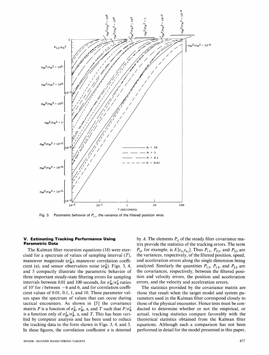
Fig. 3.
Parametric behavior of P, 1, the variance of the filtered position error.
V. Estimating Tracking Performance Using
Parametric Data
The Kalman filter recursion equations (18) were exer-
cised for a spectrum of values of sampling interval (T),
maneuver magnitude (a'), maneuver correlation coeffi-
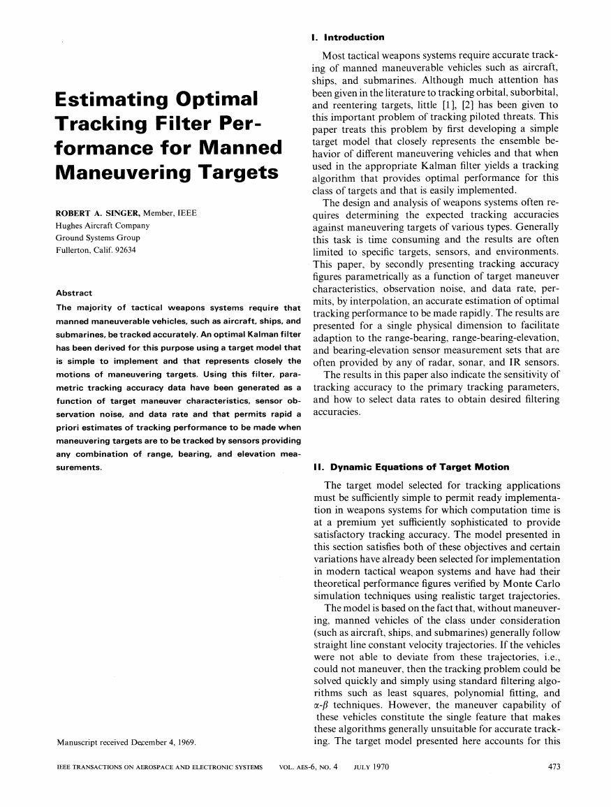
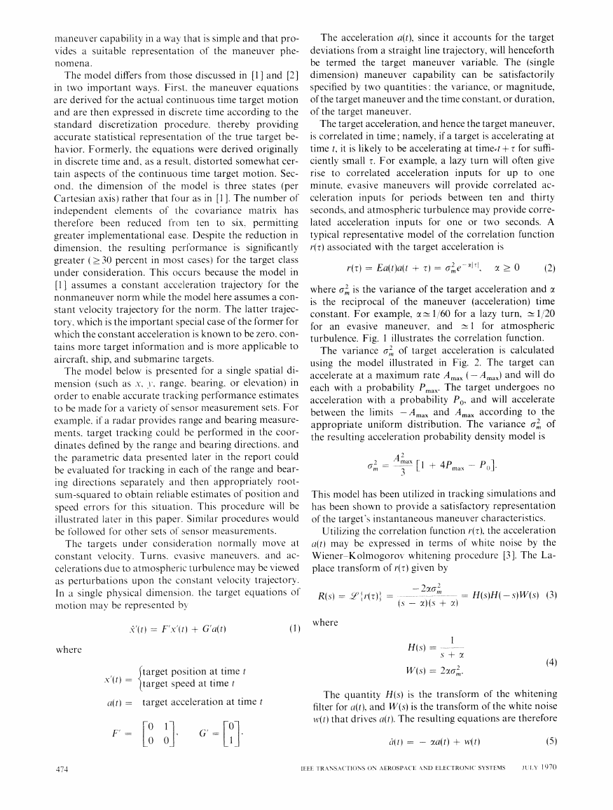
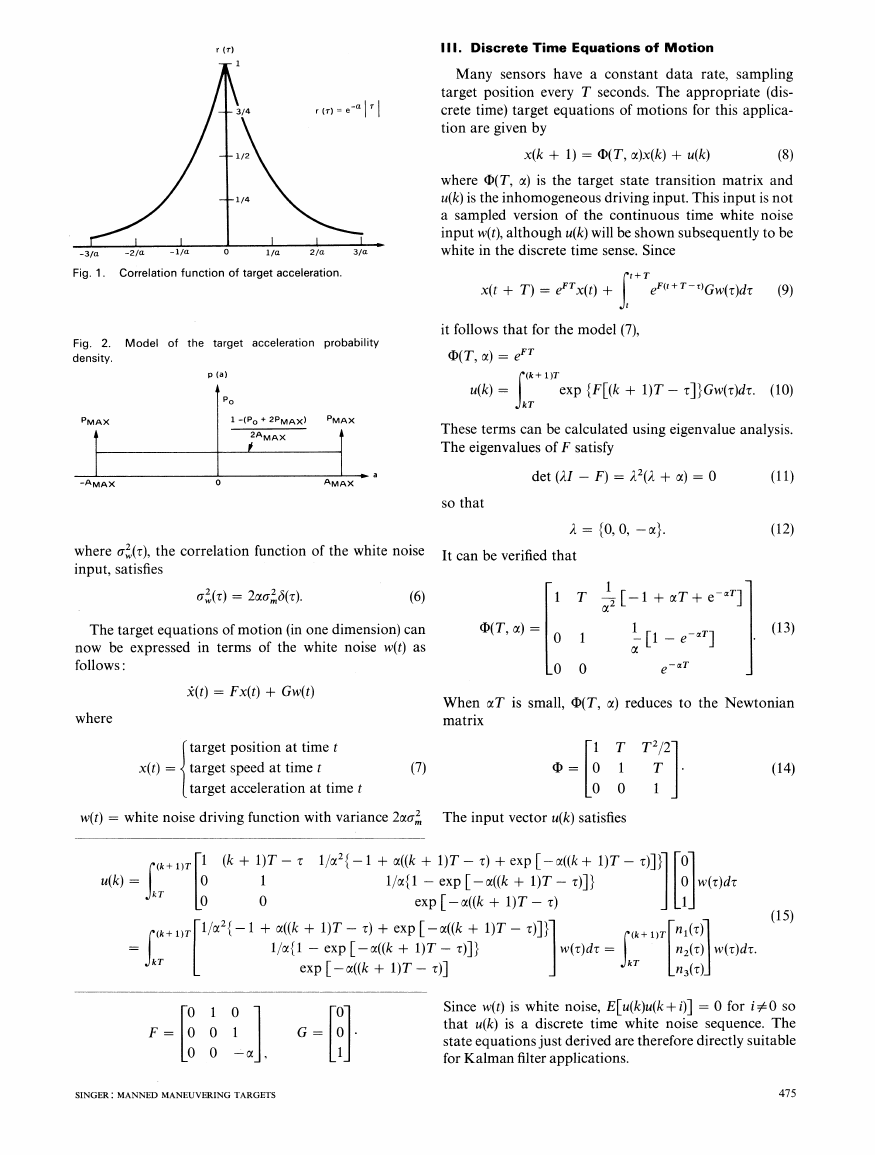
cient (a), and sensor observation noise (a'). Figs. 3, 4,
and 5 compactly illustrate the parametric behavior of
three important steady-state filtering errors for sampling
intervals between 0.01 and 100 seconds, for a2 /a2 ratios
of 1O0 for i between -6 and 6, and for correlation coeffi-
cient values of 0.01, 0.1, 1, and 10. These parameter val-
ues span the spectrum of values that can occur during
tactical encounters. As shown in [5] the covariance
matrix P is a function of 42, a2
, and T such that pIC2
is a function only of C2 /C2, a, and T. This has been veri-
fied by computer analysis and has been used to reduce
the tracking data to the form shown in Figs. 3, 4, and 5.
In these figures, the correlation coefficient cx is denoted
by A. The elements Pij of the steady filter covariance ma-
trix provide the statistics of the tracking errors. The term
Pij, for example, is E[8exig]. Thus P11, P22, and P33 are
the variances, respectively, of the filtered position, speed,
and acceleration errors along the single dimension being
analyzed. Similarly the quantities P12, P13, and P23 are
the covariances, respectively, between the filtered posi-
tion and velocity errors, the position and acceleration
errors, and the velocity and acceleration errors.
The statistics provided by the covariance matrix are
those that result when the target model and system pa-
rameters used in the Kalman filter correspond closely to
those of the physical encounter. Hence tests must be con-
ducted to determine whether or not the empirical, or
actual, tracking statistics compare favorably with the
theoretical statistics obtained from the Kalman filter
equations. Although such a comparison has not been
performed in detail for the model presented in this paper,
SINGER: MANNED MANEUVERING TARGETS
477
�
1010 F
1 09 [-
F---
r----
r
108
A -- 10
A
1
A -=0.1
A =O.l
J A1 21,P4
106
I UM2/R-2 io
M21( R2
102
Om2laR2 --1
aM2/0(R2
10-2
j aM2/aR2
10-4
(jM2/GR2 = 10-
-6
GM2/R2 = 106
aM2/0bgR2 = 104 |
0M2/aR2
102
102
10
1
GM2/MR2 =1 { 10- 1
0M2/ R2
10-2 {102
0M2/0R2 = 10-4 f
a2/aR2 = 10-6
10-3
1 o-4
l10-5
10-2
10o1
1
10
100
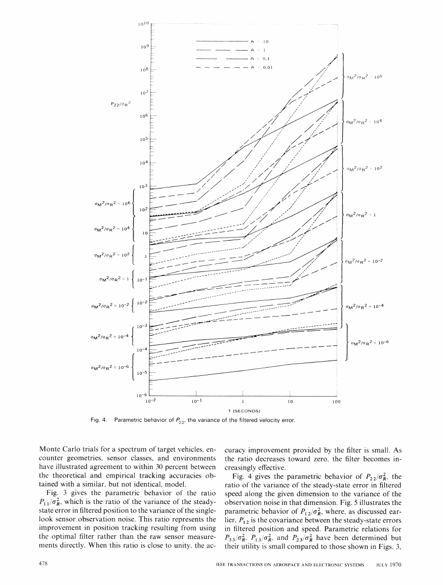
Fig. 4.
Parametric behavior of P22, the variance of the filtered velocity error.
T (SECONDS)
Fig.
Monte Carlo trials for a spectrum of target vehicles, en-
counter geometries, sensor classes, and environments
have illustrated agreement to within 30 percent between
the theoretical and empirical tracking accuracies ob-
tained with a similar, but not identical, model.
3 gives the parametric behavior of the ratio
P1 11U, which is the ratio of the variance of the steady-
state error in filtered position to the variance of the single-
look sensor observation noise. This ratio represents the
improvement in position tracking resulting from using
the optimal filter rather than the raw sensor measure-
ments directly. When this ratio is close to unity. the ac-
curacy improvement provided by the filter is small. As
the ratio decreases toward zero, the filter becomes in-
creasingly effective.
Fig. 4 gives the parametric behavior of P22/UR, the
ratio of the variance of the steady-state error in filtered
speed along the given dimension to the variance of the
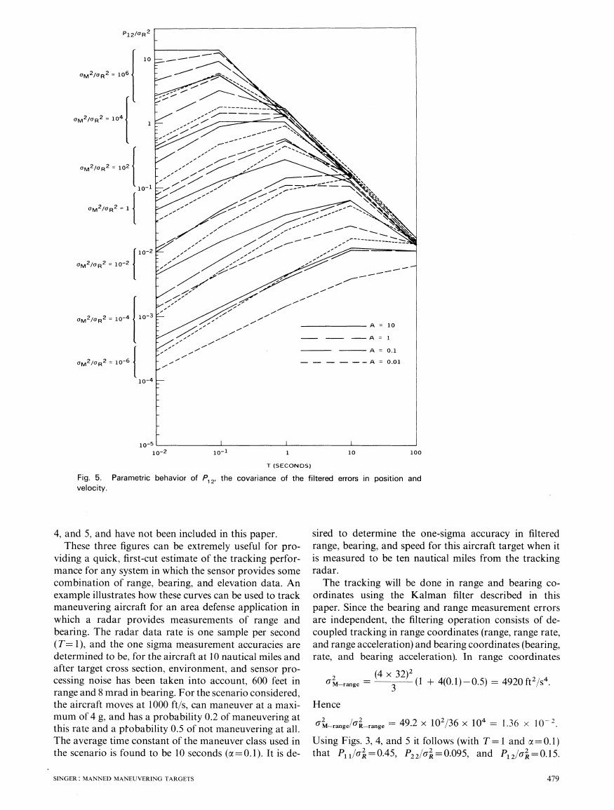
observation noise in that dimension. Fig. 5 illustrates the
parametric behavior of P12IU2, where, as discussed ear-
lier, P1 2 is the covariance between the steady-state errors
in filtered position and speed. Parametric relations for
P332 P/3/2 and P23/2 have been determined but
their utility is small compared to those shown in Figs. 3,
478
IEEE TRANSACTIONS ON AEROSPACE AND ELECTRONIC SYSTEMS
JULY 1970
�
aM2/gR2
0M2/gR2 = 1
0M2/a R2
aM2/gR2 = 1l
aM2/aR2 = 1(
0M2/IR2 = 1(
10-5
10-2
lo-'
1
10
100
T (SECONDS)
Fig. 5.
velocity.
Pa
3rametric behavior of P1 2' the
covariance of the filtered errors in position and
4, and 5, and have not been included in this paper.
These three figures can be extremely useful for pro-
viding a quick, first-cut estimate of the tracking perfor-
mance for any system in which the sensor provides some
combination of range, bearing, and elevation data. An
example illustrates how these curves can be used to track
maneuvering aircraft for an area defense application in
which a radar provides measurements of range and
bearing. The radar data rate is one sample per second
(T= 1), and the one sigma measurement accuracies are
determined to be, for the aircraft at 10 nautical miles and
after target cross section, environment, and sensor pro-
cessing noise has been taken into account, 600 feet in
range and 8 mrad in bearing. For the scenario considered,
the aircraft moves at 1000 ft/s, can maneuver at a maxi-
mum of 4 g, and has a probability 0.2 of maneuvering at
this rate and a ptobability 0.5 of not maneuvering at all.
The average time constant of the maneuver class used in
the scenario is found to be 10 seconds (o =0.1). It is de-
sired to determine the one-sigma accuracy in filtered
range, bearing, and speed for this aircraft target when it
is measured to be ten nautical miles from the tracking
radar.
The tracking will be done in range and bearing co-
ordinates using the Kalman filter described in this
paper. Since the bearing and range measurement errors
are independent, the filtering operation consists of de-
coupled tracking in range coordinates (range, range rate,
and range acceleration) and bearing coordinates (bearing,
rate, and bearing acceleration). In range coordinates
2M-range
3
(1 + 4(0.1) -0.5) = 4920 ft /s
Hence
2
M-range/ R-range
2
49.2 x
102
/36 x 10 = 1.36 x
10 2
Using Figs. 3, 4, and 5 it follows (with T= 1 and oc=0.1)
that P11/C2 = 0.45, P22
= 0.095, and P12/C = 0.15.
SINGER: MANNED MANEUVERING TARGETS
479
�
3.
Hence P11(range) -16.2 x 104 ft2 P2 1range)342x l04
5.3 x l04ft2xs2 In bearing co-
ft2 S4, and P12(range)
4920 60 0006
=
M bearin
ordinates,
so that aM-
1.36 x 10
g
i range range
'aring 7R bearng- 1.36 X 10
4. and 5,
)2 2.13x 10
Using Figs.
(8x 10
follows that P11
Hence
P2
PI (bearing)- 30.1 X It)
it
01.I 12lP,17.
P-P2(bearing)
rad
10.85 rad2 i2
bearingg)
7.03 x 10 6 rad2 < and P,
The stanidard deviation of the filtered range accuracv is
402 ft. and the standard derivation of the
P1 grange)
filtered bearing accuracy is > P1
5.5 mrad.
The target speed t, is given by v-v V+R2 r
where
1R is target range rate, R is target range,. and ivo is target
bearing rate. Hence
(bearing)
- 0.47
u
(
VRi-R -4- Rr piR -± R u06u0
6t
The variance of the speed estimate is therefore
s*peed =E(ed )2
|VP7i2(range) t R2jP1 1(range)
2R l R0 P1 2(range) + R4u P22(bearing)j
This expression accounts for the independence of range
tiu0 as the
and bearing errors, and treats 6J1R, 6R. and
errors in the filtered values of range rate, range, and
bearing rate, respectively. For a 1000 ft/s target (u,
1000)
moving on a course such that VR= Ru0 707 ft/s,
it
follows that:
used as above to provide the statistics of the S-seconds-
ahead target prediction errors.
VI. Tracking Accuracy Sensitivities
Figs. 3 and 4 illustrate the sensitivity of the errors in
filtered position and velocity to the four primary tracking
parameters: a',. u. a. and T. As such they provide
another important design tool to the tracking engineer
who must frequently answer questions regarding trade-
offs between tracking accuracy and parameter value
changes.
The data rate is the parameter most easily and there-
fore most frequently varied to improve tracking perfor-
mance. The figures show that filtering accuracy increases
as the data rate increases (T decreases). and that, in fact,
as the data rate becomes unbounded (FT-+0). the filtering
errors vanish. This occurs because for extremely short
periods of time the target exhibits essentially straight line
mnotion. Since with high data rates many measurements
are received during these periods, the filter behaves as a
least sqLuares filter being used to track nonmaneuvering
vehicles, and the tracking errors vanish. As the data rate
decreases (T-). the uncertainties caused by target
maneuver become increasingly important. and the track-
ing accuracy decreases. In the case of filtered velocity, the
tracking errors increase without bound as 7I increases,
primarily because during long periods of time, target
maneuvers can result in very large changes of target
speed. In the case of filtered position. the accuracy can
decrease only to the level of the raw single-look measure-
Sspeed = 0.707X Th2(range) + UJP1 l(range) + 2u6P12(range) + R2p2(bearing)
= 0.707
3.42 x 10⁴ + (0 0 (16.2 x 10⁴) +
2
(707
60 000
1414
60 000ft/
(5.3 x 10⁴) + (60000)2(703 x 10 6)
= 188 ft/ s,
or 18.8 percent of the target speed.
The tracking accuracies associated with predicting
target coordinates for a time S after receipt of the last
data point can also be determined by the procedure de-
veloped here. The optimal prediction equations are, in
each dimension,
X(k + Slk) -b(S, a')(k k)
(26)
and the corresponding prediction error covariance
matrix satisfies
P(k + S/k) = (S, sx)P(k k)qK(S, oa) + Q(S, x).
(27)
In this equation, the elements Pt1, Pl2, P2,2 etc., of the
covariance matrix for the filtered estimates of targets co-
ordinates, etc. can be determined directly using Figs. 3, 4,
and 5. The matrices 4(S, Y.) and Q(S, ix) are given by (13)
and (19), and once calculated can be used to obtain the
matrix P(k+S/k). The elements of this matrix are then
ment accuracy since this is the position uncertainty at
receipt of each data point.
For prediction purposes, however, the benefits of re-
ducing the data rate are not nearly so great. As (27)
shows., when predicting a fixed time S ahead., the term
Q(S, oc) always appears in the prediction error covariance
matrix P(k + Slk) so that even if the data rate is increased
to the point that the filtering error covariance matrix
P(k/k) vanishes, the prediction errors only reach a non-
zero, often not small, lower limit. This result is particu-
larly important for trajectory and orbit prediction calcu-
lations when fixed finite time period predictions are
required, and must be taken into account before a data
rate is selected.
The figures show that for the regions where filtering
improves tracking performance (P11crI< 1), the sensi-
tivity of P11o/
to T is approximately a factor of 5 in
Pi1URa per decade of T. The sensitivity of P221cr
to T
varies between a factor of 1.2/decade and 3 decades/
48()
IEEE TRANSACTFIONS ON AEROSPACE AND ELECTRONIC SYSTrEMS
JUILY 1970
�


 2023年江西萍乡中考道德与法治真题及答案.doc
 2012年重庆南川中考生物真题及答案.doc
 2013年江西师范大学地理学综合及文艺理论基础考研真题.doc
 2020年四川甘孜小升初语文真题及答案I卷.doc
 2020年注册岩土工程师专业基础考试真题及答案.doc
 2023-2024学年福建省厦门市九年级上学期数学月考试题及答案.doc
 2021-2022学年辽宁省沈阳市大东区九年级上学期语文期末试题及答案.doc
 2022-2023学年北京东城区初三第一学期物理期末试卷及答案.doc
 2018上半年江西教师资格初中地理学科知识与教学能力真题及答案.doc
 2012年河北国家公务员申论考试真题及答案-省级.doc
 2020-2021学年江苏省扬州市江都区邵樊片九年级上学期数学第一次质量检测试题及答案.doc
 2022下半年黑龙江教师资格证中学综合素质真题及答案.doc