AN INTRODUCTION TO
OPTIMIZATION
SOLUTIONS MANUAL
Fourth Edition
Edwin K. P. Chong and Stanislaw H. ˙Zak
A JOHN WILEY & SONS, INC., PUBLICATION
�
1. Methods of Proof and Some Notation
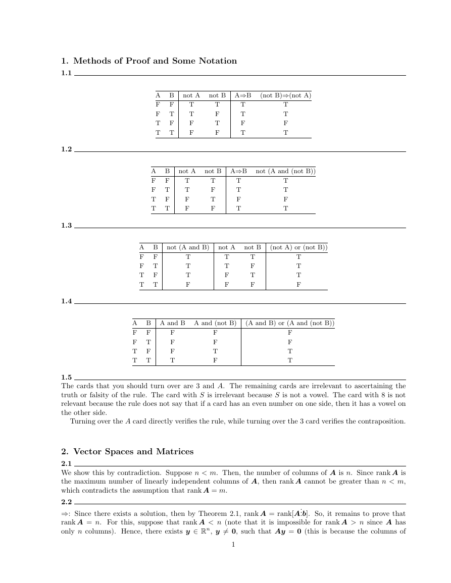
1.1
A B not A not B A⇒B (not B)⇒(not A)
F
F
F T
T F
T T
T
F
T
F
T
T
F
T
T
T
F
F
T
T
F
T
1.2
1.3
1.4
A B not A not B A⇒B not (A and (not B))
F
F
F T
T F
T T
T
F
T
F
T
T
F
T
T
T
F
T
T
T
F
F
A B not (A and B)
F
F
F T
T F
T T
T
T
T
F
not A not B (not A) or (not B))
T
T
F
F
T
F
T
F
T
T
T
F
A B A and B A and (not B)
F
F
F T
T F
T T
F
F
T
F
F
F
F
T
(A and B) or (A and (not B))
F
F
T
T
1.5
The cards that you should turn over are 3 and A. The remaining cards are irrelevant to ascertaining the
truth or falsity of the rule. The card with S is irrelevant because S is not a vowel. The card with 8 is not
relevant because the rule does not say that if a card has an even number on one side, then it has a vowel on
the other side.
Turning over the A card directly verifies the rule, while turning over the 3 card verifies the contraposition.
2. Vector Spaces and Matrices
2.1
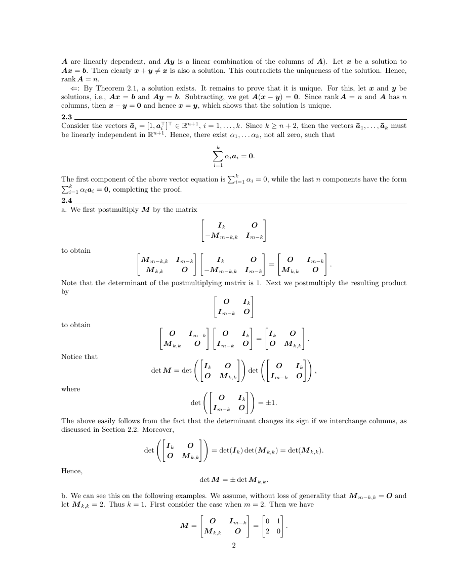
We show this by contradiction. Suppose n < m. Then, the number of columns of A is n. Since rank A is
the maximum number of linearly independent columns of A, then rank A cannot be greater than n < m,
which contradicts the assumption that rank A = m.
2.2
...b]. So, it remains to prove that
⇒: Since there exists a solution, then by Theorem 2.1, rank A = rank[A
rank A = n. For this, suppose that rank A < n (note that it is impossible for rank A > n since A has
only n columns). Hence, there exists y ∈ Rn, y 6= 0, such that Ay = 0 (this is because the columns of
1
�
A are linearly dependent, and Ay is a linear combination of the columns of A). Let x be a solution to
Ax = b. Then clearly x + y 6= x is also a solution. This contradicts the uniqueness of the solution. Hence,
rank A = n.
⇐: By Theorem 2.1, a solution exists. It remains to prove that it is unique. For this, let x and y be
solutions, i.e., Ax = b and Ay = b. Subtracting, we get A(x − y) = 0. Since rank A = n and A has n
columns, then x − y = 0 and hence x = y, which shows that the solution is unique.
2.3
Consider the vectors ¯ai = [1, a>
be linearly independent in Rn+1. Hence, there exist α1, . . . αk, not all zero, such that
i ]> ∈ Rn+1, i = 1, . . . , k. Since k ≥ n + 2, then the vectors ¯a1, . . . , ¯ak must
i=1 αi = 0, while the last n components have the form
Note that the determinant of the postmultiplying matrix is 1. Next we postmultiply the resulting product
by
αiai = 0.
i=1
i=1 αiai = 0, completing the proof.
kX
The first component of the above vector equation isPk
Pk
a. We first postmultiply M by the matrix "
#"
−M m−k,k
to obtain
"
2.4
I k
M m−k,k
I m−k
M k,k
O
I k
−M m−k,k
O
I m−k
"
=
#
.
O
I m−k
M k,k
O
"
#"
O
I k
I m−k O
O
I k
I m−k O
O
I k
O M k,k
#
#!
.
#
#
O
I m−k
#
#
"
"
=
#!
#!
det
det M = det
O
I k
O M k,k
O
I k
I m−k O
,
O
I k
I m−k O
= ±1.
to obtain
Notice that
where
"
O
M k,k
I m−k
O
"
"
det
#!
"
O
I k
O M k,k
The above easily follows from the fact that the determinant changes its sign if we interchange columns, as
discussed in Section 2.2. Moreover,
det
Hence,
= det(I k) det(M k,k) = det(M k,k).
det M = ± det M k,k.
b. We can see this on the following examples. We assume, without loss of generality that M m−k,k = O and
let M k,k = 2. Thus k = 1. First consider the case when m = 2. Then we have
"
M =
O
I m−k
M k,k
O
2
#
"
#
=
0
2
1
0
.
�
Thus,
Next consider the case when m = 3. Then
"
#
det
O
I m−k
M k,k
O
= det
det M = −2 = det (−M k,k) .
...
...
···
...
0
0
···
2
1
0
···
0
0
1
···
0
= 2 6= det (−M k,k) .
Therefore, in general,
det M 6= det (−M k,k)
However, when k = m/2, that is, when all sub-matrices are square and of the same dimension, then it is
true that
det M = det (−M k,k) .
See [121].
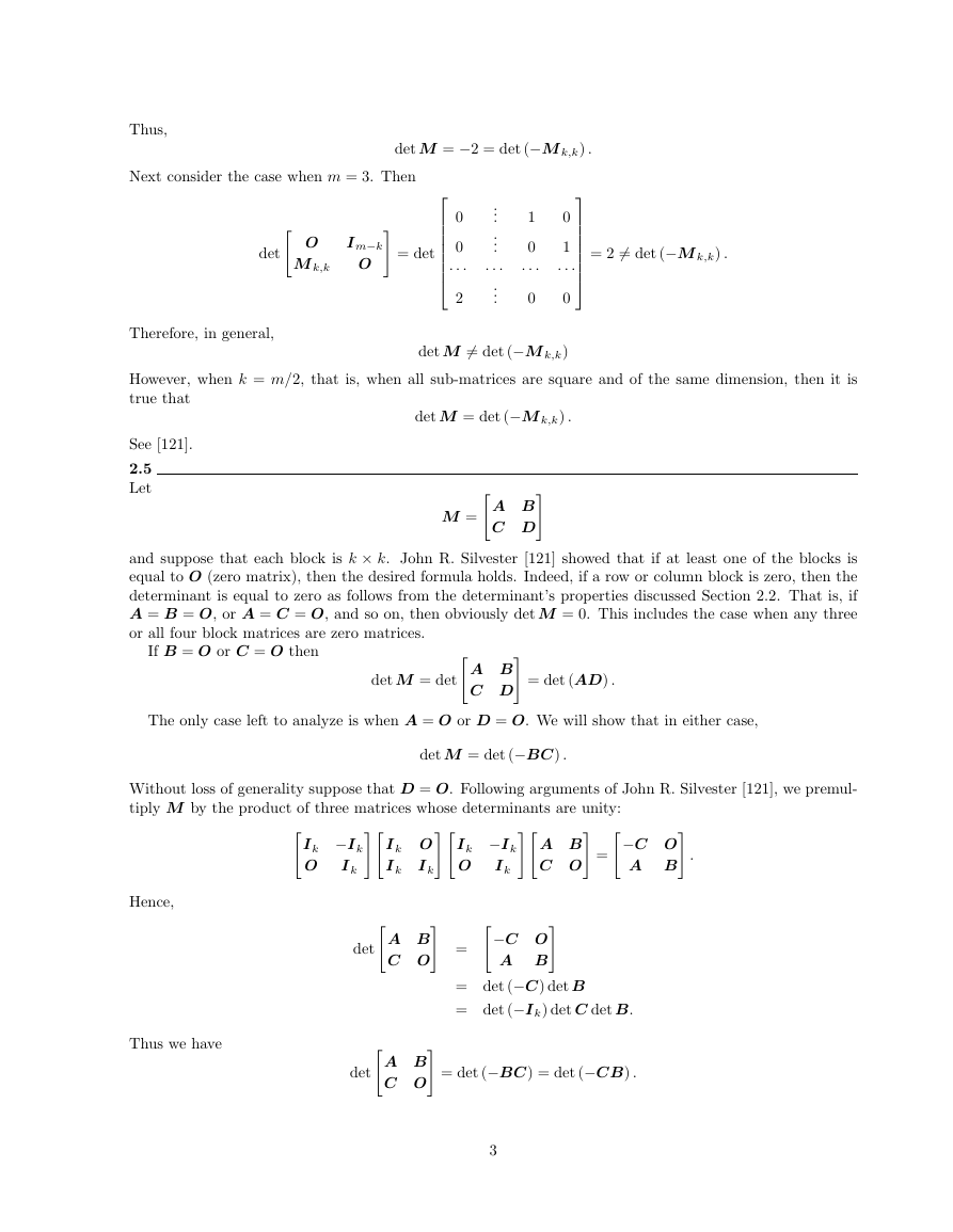
2.5
Let
"
#
A B
C D
M =
and suppose that each block is k × k. John R. Silvester [121] showed that if at least one of the blocks is
equal to O (zero matrix), then the desired formula holds. Indeed, if a row or column block is zero, then the
determinant is equal to zero as follows from the determinant’s properties discussed Section 2.2. That is, if
A = B = O, or A = C = O, and so on, then obviously det M = 0. This includes the case when any three
or all four block matrices are zero matrices.
If B = O or C = O then
"
#
A B
C D
det M = det
= det (AD) .
The only case left to analyze is when A = O or D = O. We will show that in either case,
det M = det (−BC) .
Without loss of generality suppose that D = O. Following arguments of John R. Silvester [121], we premul-
tiply M by the product of three matrices whose determinants are unity:
"
#"
#"
I k −I k
O I k
I k O
I k
I k
I k −I k
O I k
#"
#
"−C O
#
A B
.
A B
C O
=
Hence,
Thus we have
"
det
#
A B
C O
"
det
#
A B
C O
"−C O
#
A B
=
= det (−C) det B
= det (−I k) det C det B.
= det (−BC) = det (−CB) .
3
�
2.6
We represent the given system of equations in the form Ax = b, where
"
#
A =
2
1
1
1
1 −2 0 −1
,
x =
and
b =
Using elementary row operations yields
"
"
A =
2
1
1
1
1 −2 0 −1
1
1
1
0 −3 −2 −2
2
[A, b] =
1
1
1 −2
1
2
1
0 −1 −2
→
1
1
1
0 −3 −2 −2 −3
2
1
,
x1
x2
x3
x4
#
→
"
#
"
"
#
.
1
−2
#
,
and
#
,
from which rank A = 2 and rank[A, b] = 2. Therefore, by Theorem 2.1, the system has a solution.
We next represent the system of equations as
−2 + x4
Assigning arbitrary values to x3 and x4 (x3 = d3, x4 = d4), we get
1
1
1 −2
x1
x2
=
1 − 2x3 − x4
"
#"
#
"
#
#
"
#
x1
x2
=
=
= −1
3
.
"
1 − 2
1
1
1 −2
−1
1
3 d3 − 1
3 d4
3 d3 − 2
3 d4
#"
#
d3 +
#−1"
"−2 −1
" − 4
=
−a
−a if a < 0
if a = 0
if a > 0
− 4
3− 2
3
1
0
0
−(−a)
=
0
a
= |a|.
| − a| =
if −a > 0
if −a = 0
if −a < 0
1 − 2x3 − x4
−2 + x4
1 − 2x3 − x4
−2 + x4
#
d4 +
,
0
1
0
0
− 1
3− 2
3
0
1
Therefore, a general solution is
=
x1
x2
x3
x4
− 4
3 d3 − 1
3 d4
1 − 2
3 d3 − 2
3 d4
d3
d4
where d3 and d4 are arbitrary values.
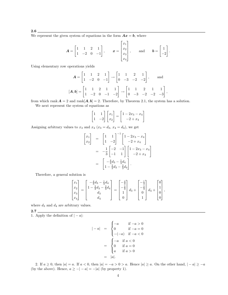
2.7
1. Apply the definition of | − a|:
2. If a ≥ 0, then |a| = a. If a < 0, then |a| = −a > 0 > a. Hence |a| ≥ a. On the other hand, | − a| ≥ −a
(by the above). Hence, a ≥ −| − a| = −|a| (by property 1).
4
�
3. We have four cases to consider. First, if a, b ≥ 0, then a + b ≥ 0. Hence, |a + b| = a + b = |a| + |b|.
Second, if a, b ≥ 0, then a + b ≤ 0. Hence |a + b| = −(a + b) = −a − b = |a| + |b|.
Third, if a ≥ 0 and b ≤ 0, then we have two further subcases:
1. If a + b ≥ 0, then |a + b| = a + b ≤ |a| + |b|.
2. If a + b ≤ 0, then |a + b| = −a − b ≤ |a| + |b|.
The fourth case, a ≤ 0 and b ≥ 0, is identical to the third case, with a and b interchanged.
4. We first show |a − b| ≤ |a| + |b|. We have
|a − b| = |a + (−b)|
≤ |a| + | − b|
= |a| + |b|
by property 3
by property 1.
To show ||a|−|b|| ≤ |a− b|, we note that |a| = |a− b+ b| ≤ |a− b|+|b|, which implies |a|−|b| ≤ |a− b|. On the
other hand, from the above we have |b| − |a| ≤ |b − a| = |a − b| by property 1. Therefore, ||a| − |b|| ≤ |a − b|.
5. We have four cases. First, if a, b ≥ 0, we have ab ≥ 0 and hence |ab| = ab = |a||b|. Second, if a, b ≤ 0,
we have ab ≥ 0 and hence |ab| = ab = (−a)(−b) = |a||b|. Third, if a ≤ 0, b ≤ 0, we have ab ≤ 0 and hence
|ab| = −ab = a(−b) = |a||b|. The fourth case, a ≤ 0 and b ≥ 0, is identical to the third case, with a and b
interchanged.
6. We have
|a + b| ≤ |a| + |b|
≤ c + d.
by property 3
7. ⇒: By property 2, −a ≤ |a| and a ≤ |a. Therefore, |a| < b implies −a ≤ |a| < b and a ≤ |a| < b.
⇐: If a ≥ 0, then |a| = a < b. If a < 0, then |a| = −a < b.
For the case when “<” is replaced by “≤”, we simply repeat the above proof with “<” replaced by “≤”.
8. This is simply the negation of property 7 (apply DeMorgan’s Law).
y = (Qx)>(Qy) = x>Q2y,
"
#
1
1
1
2
.
2.8
Observe that we can represent hx, yi2 as
hx, yi2 = x>
"
#
2
3
3
5
where
Note that the matrix Q = Q> is nonsingular.
1. Now, hx, xi2 = (Qx)>(Qx) = kQxk2 ≥ 0, and
Q =
hx, xi2 = 0 ⇔ kQxk2 = 0
⇔ Qx = 0
⇔ x = 0
since Q is nonsingular.
2. hx, yi2 = (Qx)>(Qy) = (Qy)>(Qx) = hy, xi2.
3. We have
hx + y, zi2 = (x + y)>Q2z
= x>Q2z + y>Q2z
= hx, zi2 + hy, zi2.
5
�
4. hrx, yi2 = (rx)>Q2y = rx>Q2y = rhx, yi2.
2.9
We have kxk = k(x− y) + yk ≤ kx− yk +kyk by the Triangle Inequality. Hence, kxk−kyk ≤ kx− yk. On
the other hand, from the above we have kyk − kxk ≤ ky − xk = kx − yk. Combining the two inequalities,
we obtain |kxk − kyk| ≤ kx − yk.
2.10
Let � > 0 be given. Set δ = �. Hence, if kx − yk < δ, then by Exercise 2.9, |kxk − kyk| ≤ kx − yk < δ = �.
3. Transformations
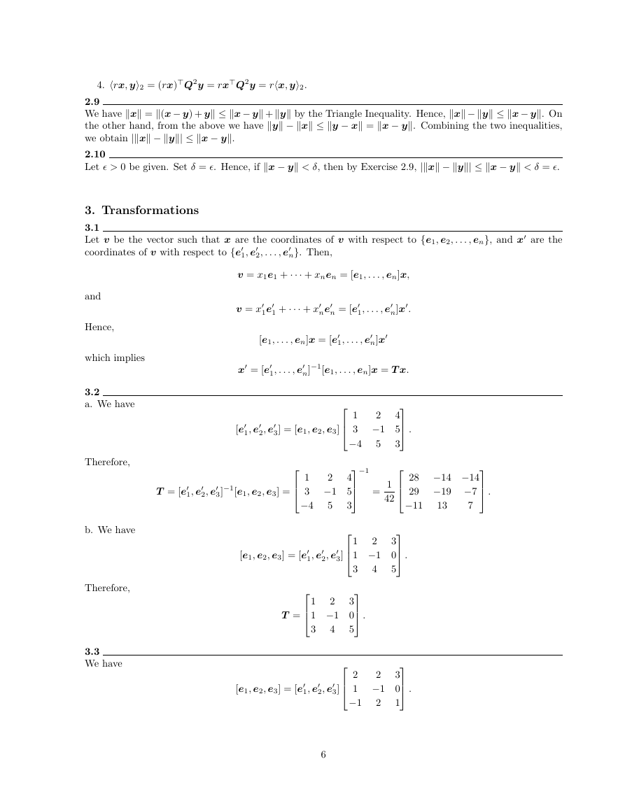
3.1
Let v be the vector such that x are the coordinates of v with respect to {e1, e2, . . . , en}, and x0 are the
coordinates of v with respect to {e0
2, . . . , e0
n}. Then,
1, e0
v = x1e1 + ··· + xnen = [e1, . . . , en]x,
and
Hence,
which implies
3.2
a. We have
Therefore,
b. We have
Therefore,
3.3
We have
v = x0
1e0
1 + ··· + x0
ne0
n = [e0
1, . . . , e0
n]x0.
[e1, . . . , en]x = [e0
1, . . . , e0
n]x0
x0 = [e0
1, . . . , e0
n]−1[e1, . . . , en]x = T x.
[e0
1, e0
2, e0
3] = [e1, e2, e3]
T = [e0
1, e0
2, e0
3]−1[e1, e2, e3] =
1
2
3 −1
−4
5
4
5
3
.
28 −14 −14
.
29 −19 −7
−11
7
13
.
=
1
42
2
1 −1
3
4
3
0
5
2
3 −1
−4
5
4
5
3
1
−1
1
.
2
3
0
5
.
3
0
1
2
1 −1
−1
2
[e1, e2, e3] = [e0
1, e0
2, e0
3]
1
2
1 −1
3
4
T =
[e1, e2, e3] = [e0
1, e0
2, e0
3]
6
�
Therefore, the transformation matrix from {e0
1, e0
3} to {e1, e2, e3} is
2, e0
2
2
1 −1
−1
2
,
3
0
1
T =
Now, consider a linear transformation L : R3 → R3, and let A be its representation with respect to
{e1, e2, e3}, and B its representation with respect to {e0
3}. Let y = Ax and y0 = Bx0. Then,
1, e0
2, e0
Hence, the representation of the linear transformation with respect to {e0
y0 = T y = T (Ax) = T A(T −1x0) = (T AT −1)x0.
2, e0
1, e0
3} is
B = T AT −1 =
.
8
−1
4
2 −13 −7
3 −10 −8
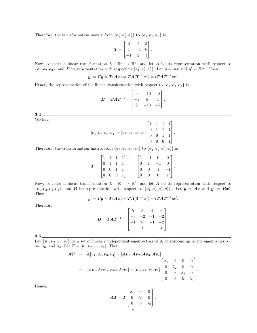
3.4
We have
3, e0
2, e0
[e0
1, e0
4] = [e1, e2, e3, e4]
1
1
1
1
0
1
1
1
0
0
1
1
1
0
0
0
4} is
Therefore, the transformation matrix from {e1, e2, e3, e4} to {e0
3, e0
2, e0
1, e0
1 −1
0
0
1 −1
0
0
1 −1
0
0
0
0
0
1
1 1
0 1
0 0
0 0
1
1
1
0
1
1
1
1
T =
−1
=
.
.
.
λ1
0
0
0
.
0
λ2
0
0
0
0
λ3
0
0
0
0
λ4
Now, consider a linear transformation L : R4 → R4, and let A be its representation with respect to
4}. Let y = Ax and y0 = Bx0.
{e1, e2, e3, e4}, and B its representation with respect to {e0
Then,
1, e0
2, e0
3, e0
y0 = T y = T (Ax) = T A(T −1x0) = (T AT −1)x0.
Therefore,
B = T AT −1 =
4
3
5
3
−3 −2 −1 −2
−1
0 −1 −2
4
1
1
1
3.5
Let {v1, v2, v3, v4} be a set of linearly independent eigenvectors of A corresponding to the eigenvalues λ1,
λ2, λ3, and λ4. Let T = [v1, v2, v3, v4]. Then,
AT = A[v1, v2, v3, v4] = [Av1, Av2, Av3, Av4]
Hence,
= [λ1v1, λ2v2, λ3v3, λ4v4] = [v1, v2, v3, v4]
AT = T
,
0
λ2
0
0
0
λ3
λ1
0
0
7
�




 2023年江西萍乡中考道德与法治真题及答案.doc
 2012年重庆南川中考生物真题及答案.doc
 2013年江西师范大学地理学综合及文艺理论基础考研真题.doc
 2020年四川甘孜小升初语文真题及答案I卷.doc
 2020年注册岩土工程师专业基础考试真题及答案.doc
 2023-2024学年福建省厦门市九年级上学期数学月考试题及答案.doc
 2021-2022学年辽宁省沈阳市大东区九年级上学期语文期末试题及答案.doc
 2022-2023学年北京东城区初三第一学期物理期末试卷及答案.doc
 2018上半年江西教师资格初中地理学科知识与教学能力真题及答案.doc
 2012年河北国家公务员申论考试真题及答案-省级.doc
 2020-2021学年江苏省扬州市江都区邵樊片九年级上学期数学第一次质量检测试题及答案.doc
 2022下半年黑龙江教师资格证中学综合素质真题及答案.doc