s
s
a
l
c
e
l
c
i
t
r
a
L
O
P
I
1
.
5
.
0
v
6
1
/
6
0
/
5
1
0
2
Published in Image Processing On Line on 2017–10–29.
Submitted on 2016–05–30, accepted on 2017–06–09.
ISSN 2105–1232 c 2017 IPOL & the authors CC–BY–NC–SA
This article is available online with supplementary materials,
software, datasets and online demo at
https://doi.org/10.5201/ipol.2017.179
The Bilateral Filter for Point Clouds
Julie Digne1, Carlo de Franchis2
1 LIRIS, CNRS UMR 5205, Universit´e Lyon 1, France (julie.digne@liris.cnrs.fr)
2 CMLA, ENS Cachan, France (carlo.de-franchis@cmla.ens-cachan.fr)
Abstract
Point sets obtained by 3D scanners are often corrupted with noise, that can have several causes,
such as a tangential acquisition direction, changing environmental lights or a reflective object
material.
It is thus crucial to design efficient tools to remove noise from the acquired data
without removing important information such as sharp edges or shape details. To do so, Fleish-
man et al. introduced a bilateral filter for meshes adapted from the bilateral filter for gray level
images. This anisotropic filter denoises a point with respect to its neighbors by considering not
only the distance from the neighbors to the point but also the distance along a normal direction.
This simple fact allows for a much better preservation of sharp edges. In this paper, we analyze
a parallel implementation of the bilateral filter adapted for point clouds.
The ANSI C++ source code permitting to reproduce results from the on-line demo is available
on the web page of the article1.
Source Code
Keywords: point set surface denoising; bilateral filtering
1
Introduction
Denoising 3D point clouds acquired by some acquisition device is one of the most important tasks of
today’s geometry processing research. Indeed, the technologies for surface acquisition have diversified:
camera-based techniques use structured light, such as a laser ray, or passive light (e.g. stereoscopy),
while some other techniques are purely laser-based (time-of-flight). In the meanwhile 3D acquisition
devices have become more popular and lower quality devices have appeared and can be obtained at
a lower cost. All these evolutions call for efficient tools to recover denoised point sets out of noisy
raw data.
This topic has been widely studied since the beginning of geometry processing research. Several
methods have been designed for meshes yet they seldom work for point clouds. One of the most
1https://doi.org/10.5201/ipol.2017.179
Julie Digne, Carlo de Franchis, The Bilateral Filter
https://doi.org/10.5201/ipol.2017.179
for Point Clouds,
Image Processing On Line, 7 (2017), pp. 278–287.
�
The Bilateral Filter for Point Clouds
widely used approaches, surface fairing, moves the vertices of the mesh in a motion governed by the
heat equation
∂x
∂t
= λ∆x.
(1)
Where x is the coordinate function. However estimating the Laplacian of a surface is a difficult
problem. In 1995, Taubin proposed a signal-based approach to surface fairing by introducing the
umbrella operator [11]: a noisy vertex is replaced by a linear combination of the positions of its
one-ring neighbors (vertices linked by an edge to the center vertex). This approach is widely used
and several variations have been proposed such as a scale dependent umbrella operator [2]. In the
meanwhile, the results on Laplacian discretization for surface meshes gave rise to a whole thread of
work dealing with Laplacian eigenfunctions and how they can be used to smooth the surface, in the
spirit of the Fourier Transform ([7], [13]).
Yet these methods remain to a certain extent isotropic: points lying on an edge are filtered no
differently than the other parts of the shape, which can over-smooth features that one might want to
preserve. To overcome this limitation, several methods have been proposed for an anisotropic fairing
of surfaces ([8], [10]). Among those methods the bilateral filter for meshes proves very efficient.
The concept of bilateral filtering was introduced for images by Tomasi et al. [12], although it
was already well defined under a different name in 1985 in a book by Yaroslavsky [14]. Instead of
denoising a pixed by considering the color values of its euclidean neighbors, it considers the color
values of the neighbors that are close both in position and in color value. This concept was adapted
to the denoising of meshes by Fleishman et al. [6], and can be extended to point clouds easily, as will
be explained in this paper.
The remainder of this paper is divided as follows: the rest of this introduction presents the input
data. Then the bilateral filter is described in Section 2, its implementation is detailed (Section 3)
as well as the proposed parallelization (Section 4). In Section 5, we comment upon the choice of
parameters and give some technical details about the code (Section 6). Finally, Section 7 presents
experiments that can be easily reproduced using the provided code.
1.1 Input Data
The input data of the algorithm is a set of unorganized points assumed to be sampled on a surface.
For visualization reasons, the provided demo2 requires consistently oriented normals (i.e. all normals
should point either inwards or outwards), but the bilateral filter has no such limitation and works
for unoriented point clouds as well. The provided code takes as input either oriented or unoriented
points, possibly with additional information such as the color, or a reflectance property.
Data Structures. The data structures used in this implementation are taken from the Ball Piv-
oting Algorithm implementation described in [3] and only slightly modified. We refer the reader to
this paper for details on methods for sorting the points in an octree and getting neighbors. The files
that are specific to this paper are BilateralFilter.h, Sample.h, Sample.cpp, FileIO.h, FileIO.cpp, and
main.cpp.
2 The Bilateral Filter
We start by reviewing the bilateral filter for meshes as it was introduced by Fleishman, Drori and
Cohen-Or in [6]. Let us first consider a meshed surface M with known normals nv at each vertex
2https://doi.org/10.5201/ipol.2017.179
279
�
Julie Digne, Carlo de Franchis
position v. Let N (v) be the 1-ring neighborhood of vertex v (i.e. the set of vertices sharing an edge
with v). Then, the filtered position of v is
where
v + δv · nv,
p∈N (v) wd(p − v)wn(|nv, p − v|)nv, p − v
p∈N (v) wd(p − v)wn(|nv, p − v|)
.
δv =
(2)
(3)
Where wd and wn are two decreasing functions.
In a nutshell, Equation (3) means that vertex v is shifted along its normal toward a weighted
average of points that are both close to v in the ambient space and close to the plane passing through
v with normal nv. To better see the link with the bilateral filter in image processing, recall that a
pixel is denoised with respect to neighboring pixels that look similar, and this similarity is computed
in terms of distance between gray values. For meshes, the similarity is measured in terms of distance
to the tangent plane. If v belongs to a sharp edge, then the only points close to the tangent plane
at v are the points on the edge: these points will be the principal contributors to the denoising of v,
thus preserving the edge.
Interestingly, another version of the bilateral filter for meshes was introduced by Jones et al. [9],
but its adaptation to point clouds is less simple since it takes into account local areas of the surface
around each point, based, for example, on a local Voronoi diagram computation.
For a non oriented point cloud P, the bilateral filter can be extended as follows:
• First a unit unoriented normal vector np is estimated for each point p via its neighbors Nr(p) =
{q ∈ P|q − p2 < r}.
• Then the point position is updated via p = p + δp · np and
q∈Nr(p) wd(q − p)wn(|np, q − p|)np, q − p
q∈Nr(p) wd(q − p)wn(|np, q − p|)
δp =
.
(4)
Where wd and wn are two decreasing functions.
In our implementation wd and wn are two centered Gaussian functions whose variance (σd and
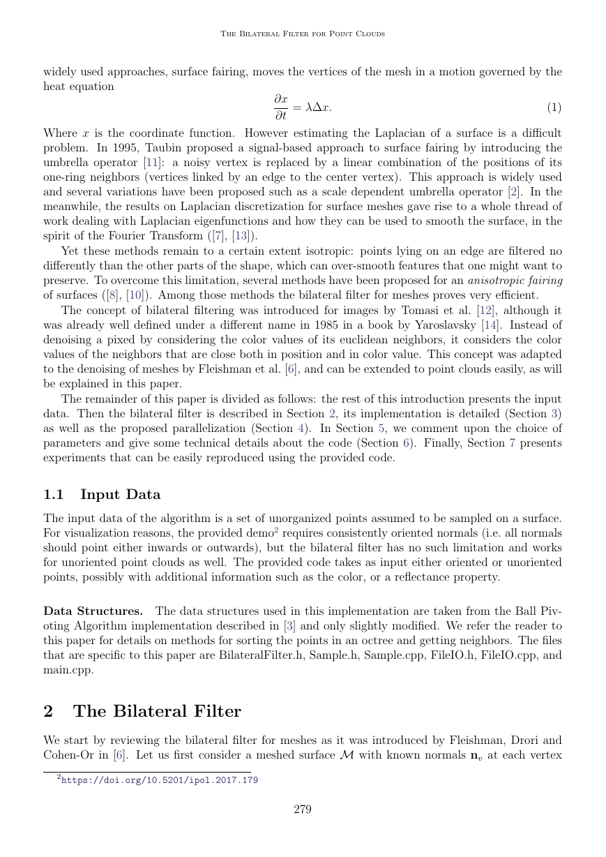
σn resp.) are chosen by the user. As can be seen on Figure 1, the weights on the distances will be
balanced by the weights on the normal distances, thus favoring nearby points that are close to the
tangent plane: the points that lie on the same side of the edge as p.
(a) Initial point p
with its neighborhood
(b) Distance weights (c) Regression plane
estimation
(d) Normal distances
|q − p, np|
(e) Normal distance
weights
Figure 1: Contributions of neighbors to the denoising of a point p in the bilateral framework. Weights are depicted in a
color scale in 1(b) and 1(e) (blue = small weights, red = large weights).
The normal np is estimated by computing the least squares regression plane of the set of neighbors
Nr(p) and setting np to be the normal to this plane. Computing the least squares regression plane is
280
ppppp�
The Bilateral Filter for Point Clouds
done trivially by computing the mean and covariance matrix of the neighbors, which yields a point
on the plane (the mean) and the normal (the eigenvector corresponding to the least eigenvalues of
the covariance matrix). Interestingly enough the orientation of the estimated normal np is irrelevant
for the computation: inverting it will yield the same denoised point p.
Implementation
3
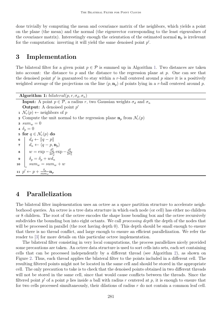
The bilateral filter for a given point p ∈ P is summed up in Algorithm 1. Two distances are taken
into account: the distance to p and the distance to the regression plane at p. One can see that
the denoised point p is guaranteed to stay within a r-ball centered around p since it is a positively
weighted average of the projections on the line (p, np) of points lying in a r-ball centered around p.
Algorithm 1: bilateral(p, r, σd, σn)
Input: A point p ∈ P, a radius r, two Gaussian weights σd and σn
Output: A denoised point p
1 Nr(p) ← neighbors of p
2 Compute the unit normal to the regression plane np from Nr(p)
3 sumw = 0
4 δp = 0
5 for q ∈ Nr(p) do
dd ← q − p
dn ← q − p, np
w = exp− d2
d
2σ2
d
δp = δp + wdn
sumw = sumw + w
exp− d2
n
2σ2
n
6
7
8
9
10
11 p ← p + δp
np
sumw
4 Parallelization
The bilateral filter implementation uses an octree as a space partition structure to accelerate neigh-
borhood queries. An octree is a tree data structure in which each node (or cell) has either no children
or 8 children. The root of the octree encodes the shape loose bouding box and the octree recursively
subdivides the bounding box into eight octants. We call processing depth the depth of the nodes that
will be processed in parallel (the root having depth 0). This depth should be small enough to ensure
that there is no thread conflict, and large enough to ensure an efficient parallelization. We refer the
reader to [3] for more details on this particular octree implementation.
The bilateral filter consisting in very local computations, the process parallelizes nicely provided
some precautions are taken. An octree data structure is used to sort cells into sets, each set containing
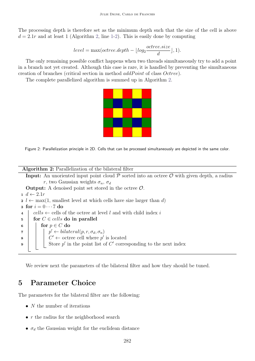
cells that can be processed independently by a different thread (see Algorithm 2), as shown on
Figure 2. Thus, each thread applies the bilateral filter to the points included in a different cell. The
resulting filtered points might not be located in the same cell and should be stored in the appropriate
cell. The only precaution to take is to check that the denoised points obtained in two different threads
will not be stored in the same cell, since that would cause conflicts between the threads. Since the
filtered point p of a point p lies inside a ball with radius r centered at p, it is enough to ensure that
for two cells processed simultaneously, their dilations of radius r do not contain a common leaf cell.
281
�
Julie Digne, Carlo de Franchis
The processing depth is therefore set as the minimum depth such that the size of the cell is above
d = 2.1r and at least 1 (Algorithm 2, line 1-2). This is easily done by computing
level = max(octree.depth − log2
octree.size
d
, 1).
The only remaining possible conflict happens when two threads simultaneously try to add a point
in a branch not yet created. Although this case is rare, it is handled by preventing the simultaneous
creation of branches (critical section in method addP oint of class Octree).
The complete parallelized algorithm is summed up in Algorithm 2.
Figure 2: Parallelization principle in 2D. Cells that can be processed simultaneously are depicted in the same color.
Algorithm 2: Parallelization of the bilateral filter
Input: An unoriented input point cloud P sorted into an octree O with given depth, a radius
Output: A denoised point set stored in the octree O.
r, two Gaussian weights σn, σd
1 d ← 2.1r
2 l ← max(1, smallest level at which cells have size larger than d)
3 for i = 0··· 7 do
cells ← cells of the octree at level l and with child index i
for C ∈ cells do in parallel
4
5
6
7
8
9
for p ∈ C do
p ← bilateral(p, r, σd, σn)
C ← octree cell where p is located
Store p in the point list of C corresponding to the next index
We review next the parameters of the bilateral filter and how they should be tuned.
5 Parameter Choice
The parameters for the bilateral filter are the following:
• N the number of iterations
• r the radius for the neighborhood search
• σd the Gaussian weight for the euclidean distance
282
�
The Bilateral Filter for Point Clouds
• σn the Gaussian weight for the distance to the tangent plane
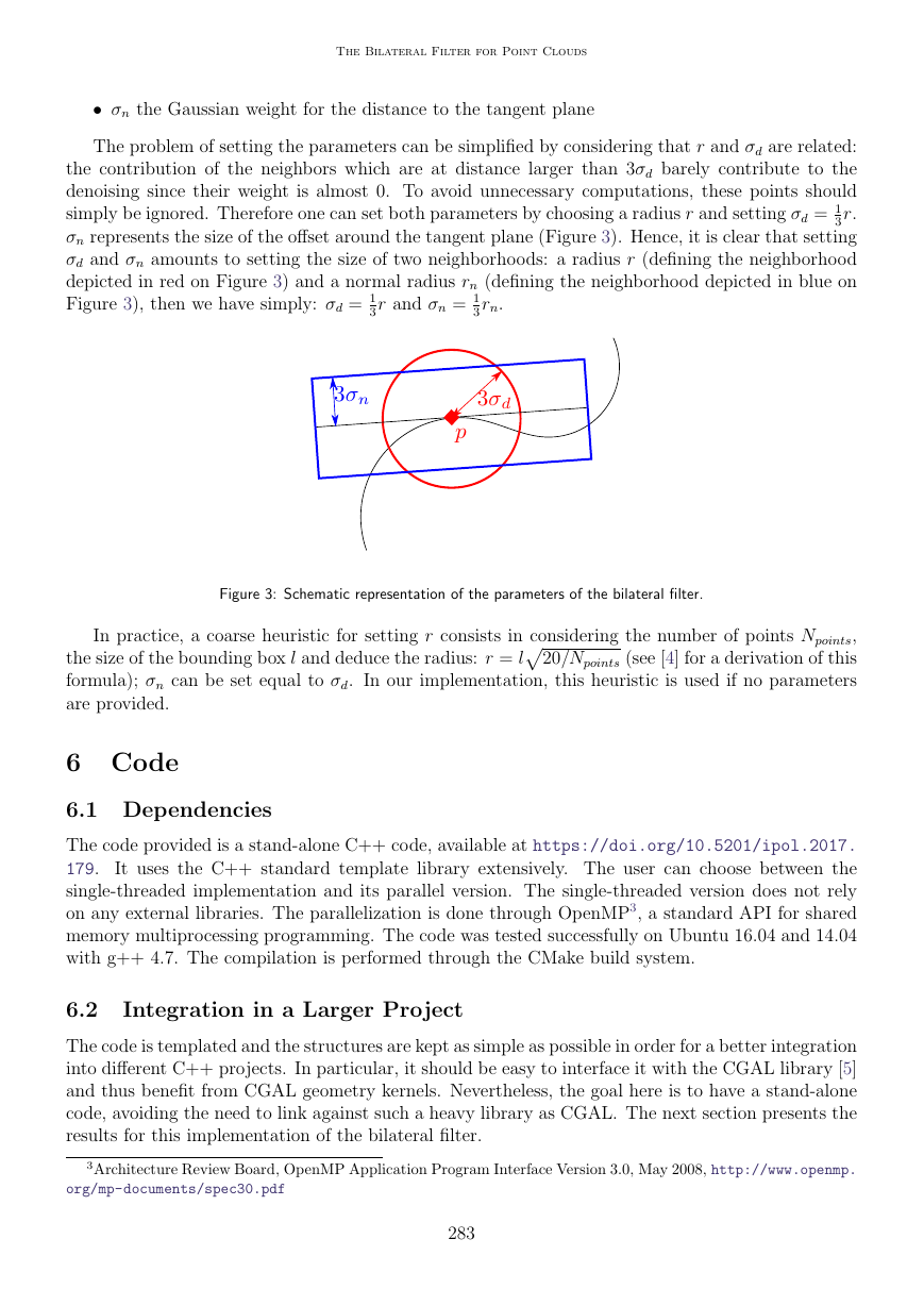
The problem of setting the parameters can be simplified by considering that r and σd are related:
the contribution of the neighbors which are at distance larger than 3σd barely contribute to the
denoising since their weight is almost 0. To avoid unnecessary computations, these points should
simply be ignored. Therefore one can set both parameters by choosing a radius r and setting σd = 1
3r.
σn represents the size of the offset around the tangent plane (Figure 3). Hence, it is clear that setting
σd and σn amounts to setting the size of two neighborhoods: a radius r (defining the neighborhood
depicted in red on Figure 3) and a normal radius rn (defining the neighborhood depicted in blue on
Figure 3), then we have simply: σd = 1
3r and σn = 1
3rn.
Figure 3: Schematic representation of the parameters of the bilateral filter.
the size of the bounding box l and deduce the radius: r = l20/Npoints (see [4] for a derivation of this
In practice, a coarse heuristic for setting r consists in considering the number of points Npoints,
formula); σn can be set equal to σd. In our implementation, this heuristic is used if no parameters
are provided.
6 Code
6.1 Dependencies
The code provided is a stand-alone C++ code, available at https://doi.org/10.5201/ipol.2017.
179.
It uses the C++ standard template library extensively. The user can choose between the
single-threaded implementation and its parallel version. The single-threaded version does not rely
on any external libraries. The parallelization is done through OpenMP3, a standard API for shared
memory multiprocessing programming. The code was tested successfully on Ubuntu 16.04 and 14.04
with g++ 4.7. The compilation is performed through the CMake build system.
6.2 Integration in a Larger Project
The code is templated and the structures are kept as simple as possible in order for a better integration
into different C++ projects. In particular, it should be easy to interface it with the CGAL library [5]
and thus benefit from CGAL geometry kernels. Nevertheless, the goal here is to have a stand-alone
code, avoiding the need to link against such a heavy library as CGAL. The next section presents the
results for this implementation of the bilateral filter.
3Architecture Review Board, OpenMP Application Program Interface Version 3.0, May 2008, http://www.openmp.
org/mp-documents/spec30.pdf
283
p3σn3σd�
Julie Digne, Carlo de Franchis
7 Experiments
For a better visualization, all point sets were first meshed using the scale space meshing algorithm
with the implementation of [4]. The parameters for this reconstruction step were always: 4 iterations
and the radius equal to half of r (the parameter for the bilateral filter).
7.1 Synthetic Examples
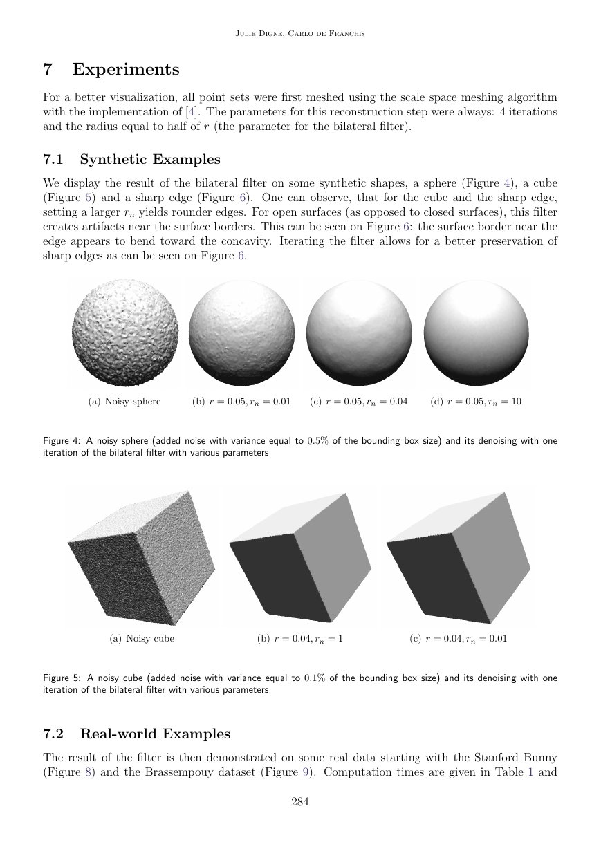
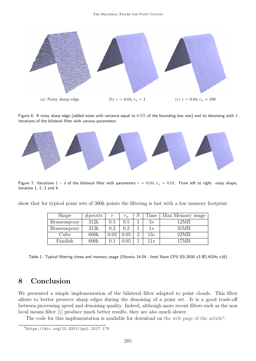
We display the result of the bilateral filter on some synthetic shapes, a sphere (Figure 4), a cube
(Figure 5) and a sharp edge (Figure 6). One can observe, that for the cube and the sharp edge,
setting a larger rn yields rounder edges. For open surfaces (as opposed to closed surfaces), this filter
creates artifacts near the surface borders. This can be seen on Figure 6: the surface border near the
edge appears to bend toward the concavity. Iterating the filter allows for a better preservation of
sharp edges as can be seen on Figure 6.
(a) Noisy sphere
(b) r = 0.05, rn = 0.01
(c) r = 0.05, rn = 0.04
(d) r = 0.05, rn = 10
Figure 4: A noisy sphere (added noise with variance equal to 0.5% of the bounding box size) and its denoising with one
iteration of the bilateral filter with various parameters
(a) Noisy cube
(b) r = 0.04, rn = 1
(c) r = 0.04, rn = 0.01
Figure 5: A noisy cube (added noise with variance equal to 0.1% of the bounding box size) and its denoising with one
iteration of the bilateral filter with various parameters
7.2 Real-world Examples
The result of the filter is then demonstrated on some real data starting with the Stanford Bunny
(Figure 8) and the Brassempouy dataset (Figure 9). Computation times are given in Table 1 and
284
�
The Bilateral Filter for Point Clouds
(a) Noisy sharp edge
(b) r = 0.04, rn = 1
(c) r = 0.04, rn = 100
Figure 6: A noisy sharp edge (added noise with variance equal to 0.5% of the bounding box size) and its denoising with 4
iterations of the bilateral filter with various parameters
Iterations 1 − 4 of the bilateral filter with parameters r = 0.04, rn = 0.01. From left to right: noisy shape,
Figure 7:
iteration 1, 2 ,3 and 4.
show that for typical point sets of 300k points the filtering is fast with a low memory footprint.
Shape
#points
Brassempouy
Brassempouy
Cube
Fandisk
312k
312k
600k
600k
r
0.5
0.2
0.03
0.1
rn N Time Max Memory usage
0.5
0.2
0.05
0.05
12MB
35MB
22MB
17MB
1
1
2
1
3s
1s
13s
11s
Table 1: Typical filtering times and memory usage (Ubuntu 14.04 - Intel Xeon CPU E5-2630 v3 @2.4GHz x16)
8 Conclusion
We presented a simple implementation of the bilateral filter adapted to point clouds. This filter
allows to better preserve sharp edges during the denoising of a point set.
It is a good trade-off
between processing speed and denoising quality. Indeed, although more recent filters such as the non
local means filter [1] produce much better results, they are also much slower.
The code for this implementation is available for download on the web page of the article4.
4https://doi.org/10.5201/ipol.2017.179
285
�


 2023年江西萍乡中考道德与法治真题及答案.doc
 2012年重庆南川中考生物真题及答案.doc
 2013年江西师范大学地理学综合及文艺理论基础考研真题.doc
 2020年四川甘孜小升初语文真题及答案I卷.doc
 2020年注册岩土工程师专业基础考试真题及答案.doc
 2023-2024学年福建省厦门市九年级上学期数学月考试题及答案.doc
 2021-2022学年辽宁省沈阳市大东区九年级上学期语文期末试题及答案.doc
 2022-2023学年北京东城区初三第一学期物理期末试卷及答案.doc
 2018上半年江西教师资格初中地理学科知识与教学能力真题及答案.doc
 2012年河北国家公务员申论考试真题及答案-省级.doc
 2020-2021学年江苏省扬州市江都区邵樊片九年级上学期数学第一次质量检测试题及答案.doc
 2022下半年黑龙江教师资格证中学综合素质真题及答案.doc