半监督式深度极限学习机，用于基于Wi-Fi的本地化.pdf

发布时间：2022-05-30 发布人：admin 分类：说明书资料大小：2.36M 资料格式：pdf 举报版权申诉

weixin_38723242-16678068-16359647678386373067.pdf-第1页.png

第1页 / 共12页

weixin_38723242-16678068-16359647678386373067.pdf-第2页.png

第2页 / 共12页

weixin_38723242-16678068-16359647678386373067.pdf-第3页.png

第3页 / 共12页

weixin_38723242-16678068-16359647678386373067.pdf-第4页.png

第4页 / 共12页

weixin_38723242-16678068-16359647678386373067.pdf-第5页.png

第5页 / 共12页

weixin_38723242-16678068-16359647678386373067.pdf-第6页.png

第6页 / 共12页

weixin_38723242-16678068-16359647678386373067.pdf-第7页.png

第7页 / 共12页

weixin_38723242-16678068-16359647678386373067.pdf-第8页.png

第8页 / 共12页

Semi-supervised deep extreme learning machine for Wi-Fi based localization

Introduction

Related works

Methodology--Semi-supervised deep extreme learning machine

A. Graph based Semi-supervised Learning

B. Deep Learning

C. Extreme Learning Machine

D. Proposed Semi-Supervised Deep Extreme Learning Machine

Performance Evaluation

A. Office environment

a) Model generation

b) Feature Extraction

c) Localization Performance

d) Man-hour Cost

B. Lobby environment

a) Feature Extraction

b) Localization Performance

Conclusion

Acknowledgement

References

Neurocomputing 166 (2015) 282–293 Contents lists available at ScienceDirect Neurocomputing journal homepage: www.elsevier.com/locate/neucom Semi-supervised deep extreme learning machine for Wi-Fi based localization Yang Gu a,b,c, Yiqiang Chen a,b,n, Junfa Liu a,b, Xinlong Jiang a,b,c a Institute of Computing Technology, Chinese Academy of Sciences, Beijing, China b Beijing Key Laboratory of Mobile Computing and Pervasive Device, Beijing, China c University of Chinese Academy of Sciences, Beijing, China a r t i c l e i n f o a b s t r a c t Article history: Received 12 September 2014 Received in revised form 29 March 2015 Accepted 2 April 2015 Communicated by: G.-B. Huang Available online 23 April 2015 Keywords: Wi-Fi indoor localization Semi-supervised learning Deep learning Extreme Learning Machine (ELM) Along with the proliferation of mobile devices and wireless signal coverage, indoor localization based on Wi-Fi gets great popularity. Fingerprint based method is the mainstream approach for Wi-Fi indoor localization, for it can achieve high localization performance as long as labeled data are sufﬁcient. However, the number of labeled data is always limited due to the high cost of data acquisition. Nowadays, crowd sourcing becomes an effective approach to gather large number of data; meanwhile, most of them are unlabeled. Therefore, it is worth studying the use of unlabeled data to improve localization performance. To achieve this goal, a novel algorithm Semi-supervised Deep Extreme Learning Machine (SDELM) is proposed, which takes the advantages of semi-supervised learning, Deep Leaning (DL), and Extreme Learning Machine (ELM), so that the localization performance can be improved both in the feature extraction procedure and in the classiﬁer. The experimental results in real indoor environments show that the proposed SDELM not only outperforms other compared methods but also reduces the calibration effort with the help of unlabeled data. & 2015 Elsevier B.V. All rights reserved. 1. Introduction Wireless localization based on Wi-Fi is quite popular, especially in indoor environment [1–3], for it does not need deploying any extra infrastructure. What is more, the widespread Access Points (APs) and smart mobile devices facilitate the development of Wi-Fi based indoor localization. To implement indoor localization, tradi- tionally, labeled data are required. In Wi-Fi localization ﬁeld, labeled data means both data and their corresponding locations (coordi- nates/classes) are known; unlabeled data means only data are available, and whose corresponding locations are unknown. Gen- erally, there are mainly two types of Wi-Fi localization methods: propagation based method and ﬁngerprint based method. The propagation based method takes the advantage of the nonlinear fading characteristics of wireless signal to set up a propagation model [1]. This kind of method can be easily implemented; however, the localization performance is not good enough for it is difﬁcult to set up an accurate propagation model in a complex and dynamic indoor environment. Compared with propagation based method, ﬁngerprint based localization method is widely adopted. “Finger- prints” are features obtained by feature extraction methods, and used to represent the corresponding locations; “localization” means n Corresponding author at: Institute of Computing Technology, Chinese Academy of Sciences, Beijing, China. http://dx.doi.org/10.1016/j.neucom.2015.04.011 0925-2312/& 2015 Elsevier B.V. All rights reserved. adopting pattern recognition method to estimate the location. Theoretically, the more the labeled data are, the better the localiza- tion performance will be. However, the calibration procedure (which is also known as the acquisition of labeled data) is always at the cost of time, man-hour and money, which leads to the limited number of labeled data. According to [4], “calibration procedures are applied in a great number of proposed location techniques and are considered to be not practical or a considerable barrier to wider adoption of such methods”. As reported [5], Ekahau [6], a commercial real-time localization system, spent $10,000 just to collect labeled data in a large ofﬁce building, which clearly veriﬁes the high cost of obtaining labeled data. In contrast to the acquisition of labeled data, the collection of unlabeled data can be carried out easily; especially when crowd sourcing is adopted. Crowd Sourcing [7,8] is a distributed model to solve problems through an open way with different participants. For indoor localization, crowd sourcing (data collection) means gathering data from heterogeneous devices [9], and most of the data are unlabeled. In order to use unlabeled data, works based on manifold learning and semi-supervised learning were proposed. These works indeed improved localization performance with unlabeled data; however, they paid less attention to the problem caused by crowd sourcing. After data have been collected for localization system, feature extraction becomes an important step. Though Received Signal Strength (RSS) of Wi-Fi signal has real physical meaning and can

Y. Gu et al. / Neurocomputing 166 (2015) 282–293 283 be directly used as feature; the highly dynamic indoor environment and heterogeneous devices lead to severe ﬂuctuation of wireless signal, which makes this kind of direct feature less representative. Traditional indoor localization methods mainly selected features manually or extracted features by shallow networks, which cannot reﬂect Wi-Fi characteristics in complex environment well. However, a machine learning method, Deep Learning (DL) has been famous worldwide since 2006 [10]. DL learns high level features and distributed data structure, which can represent original data better than shallow feature. Though DL outperforms traditional neural networks, its training time consumption is high. While, Extreme Learning Machine (ELM) proposed in the same period as DL, is popular for fast learning speed, which can make up the time- consuming shortage of DL. Considering the analysis above, we put forward a novel localiza- tion method, Semi-supervised Deep Extreme Learning Machine (SDELM) to improve the localization performance with unlabeled data. The contribution of this work is: 1) Utilize unlabeled data to get discriminative features and better classiﬁcation ability; 2) Propose semi-supervised embedding for deep leaning network; 3) Adopt modiﬁed ELM to improve the learning speed of SDELM. The rest of this paper is organized as follows: Section II shows the related works in Wi-Fi localization ﬁeld. Section III introduces the proposed SDELM in detail. Section IV evaluates the performance of SDELM in real wireless indoor environments. And Section V con- cludes the work. 2. Related works The mainstream approach of Wi-Fi based indoor localization, ﬁngerprint based method [2,3], consists of two phases: off-line training phase and online locating phase. At training phase, features are extracted according to a certain rule, so that the relationship between features and their corresponding locations can be estab- lished, which forms a “radio map”; at online locating phase, features of unknown location are extracted with the same rule, and pattern recognition methods are used to ﬁnd the best matched locations on the “radio map”, then the ﬁnal location can be estimated by those matched locations. Two parts in ﬁngerprint based method: feature extraction and pattern recognition (classiﬁer) involve unlabeled/ labeled data, which can affect the overall localization performance. For these two parts, there are many related works. For feature extraction, it is well-known that Wi-Fi signal is ﬁckle: the unpredictable movement of people, the status of door (open/ closed), the change of temperature and humidity, the placement of objects, the type of device [11] et al., which all lead to the ﬂuctuation of Wi-Fi signal. Hence, feature extraction work of Wi-Fi can greatly affect the ﬁnal localization performance. Up till now, most ﬁngerprint methods extract shallow level information from labeled data as Wi-Fi feature. Mean value method is the commonest feature extraction method [12–15], which collected multiple RSS vectors at the same location, and averaged those vectors to form the feature. Even though RSS changes unpredictably, the mean value can, from the statistical view, reduce the unstableness of RSS. Further than mean value method, Gaussian model was put forward based on the assumption that RSS at the same location satisﬁed Gaussian distribution. [16] utilized Gaussian process to eliminate the side-effect caused by small probability RSS and outliers, and averaged high probability RSS vectors to get feature. Except for statistical feature extraction meth- ods, unsupervised machine learning method is also adopted. [17] used Principal Component Analysis (PCA) to extract Wi-Fi feature; the principal components of multi-dimension wireless signal not only offered new feature but also reduced the effect of noise. AP selection methods were also put forward, for AP is the emission source of Wi-Fi signal. [18] picked out k APs with the strongest RSS at each location as feature. [19] proposed InfoGain criterion to evaluate the merit of each AP in terms of power and selected the highest ones to form feature. Other than common feature extraction approaches, special methods were also presented to solve speciﬁc problems. To overcome the variance caused by different devices, [20] came up with a hyperbolic method, utilizing signal strength ratio instead of absolute signal strength to form feature. And to mitigate the distortion caused by human body, [21] proposed an ellipse signal attenuation model to generate an orientation-independent ﬁngerprint database. Though there were many works proposed to extract features for Wi-Fi based localization, seldom utilized unlabeled data. Besides, most of them were at shallow level, which cannot represent the Wi- Fi characteristics in complex indoor environment well. For ﬁngerprint based localization methods, pattern recognition methods (classiﬁers) are used to estimate the ﬁnal localization result, and most of the traditional methods are supervised [1]. However, considering the fact that labeled data are limited and unlabeled data are adequate, manifold learning and semi-supervised learning methods were widely adopted. Pan [22] proposed a manifold learning method to calculated users’ location and APs’ location. It ﬁrst adopted SVD based method with labeled and unlabeled data to calculate relative locations (which is a dimension reduction process), then used manifold assumption to get the absolute locations with the assist of labeled data. Pulkkinen [23] used Isomap method to reduce the feature space to a low dimension manifold space; then transformed the manifold space to location space to implement localization. By carefully selected key points to represent ﬁngerprints, this method can calibrate an entire radio map based on a small fraction of labeled data; and according to the experiment, the mean localization error was 2.0 m when there were 66 testing points. Zhang [24] presented LocMR method based on manifold regularization, which learnt the mapping from signal space to location space; the novelty of the work is that time span constraint is brought into the calculation of Laplacian matrix, so that the manifold in time domain can be maintained. In order to utilize unlabeled data, Lin [25] applied spectral decomposition of Laplacian matrix to get data representation in eigenvectors space, then added labels to unlabeled data by aligning labeled data. The result showed that only with small proportion of labeled data like 20%, the localization accuracy can reach to 75%. A semi-supervised localization method, Semi-supervised Extreme Learning Machine (SELM) [26], was put forward based on ELM, which brought graph Laplacian constraint to ELM, so that the sparsely calibrated localiza- tion system can perform well with fast learning speed. Though there are plenty of existing manifold and semi- supervised works which can improve the localization performance with unlabeled data; however, most of them are based on shallow features and do not take crowd sourcing into consideration. Therefore, considering the practical localization problems such as feature extraction and unlabeled data from crowd sourcing, we put forward SDELM method on the basis of semi-supervised learning, deep learning and ELM, so that the overall localization performance can be improved. 3. Methodology–Semi-supervised deep extreme learning machine Graph based semi-supervised learning is embedded to deep learning structure to get discriminative feature and better classiﬁca- tion boundary. To guarantee the learning speed, semi-supervised learning is evolved from ELM. Hence, in this section, we ﬁrstly

284 Y. Gu et al. / Neurocomputing 166 (2015) 282–293 goal of AE based DL is to minimize reconstruct error, making hW;b Xk Xk, which equals to minimize the loss function: # ð J W; b Þ ¼ min W;b " " 1 N XN XN i ¼ 1 i ¼ 1 1 2 ¼ min W;b 1 N brieﬂy introduce graph based semi-supervised learning, deep lean- ing, and ELM; then elaborate the proposed SDELM in detail. 3.1. A. Graph based Semi-supervised Learning Semi-supervised learning is between unsupervised learning and supervised learning, which utilizes a small amount of labeled data and a large amount of unlabeled to train a model. There are three assumptions for semi-supervised learning [27]: smoothness assump- tion, cluster assumption and manifold assumption. The smoothness assumption implies that if two points are close in a high-density region, their corresponding outputs should also be close. The cluster assumption is used to ﬁnd the boundary of each cluster, for “if points are in the same cluster, they are likely to be in the same class”, and cluster assumption can be seen as a special case of smooth assump- tion. The manifold assumption is used to avoid “the curse of dimensionality”. And semi-supervised learning should satisfy at least one of the above assumptions. Semi-supervised learning usually adopts graph based methods, data points (both labeled and unlabeled data) are the vertexes of the graph, and the goal of graph based methods can be expressed as: ! V f xið Þ; yi þλA‖f ‖2 þλI Z M arg min f 1 l f xð Þ‖∇Mf xð Þ‖2dp xð Þ ð1Þ Where M is the manifold that data lie in, and λA, λI are the parameters control the smoothness in the ambient and intrinsic spaces, l is the number of samples. Among all the graph based methods, Laplacian graph is mostly adopted, which makes (1) be approximately expressed as: V f xið Þ; yi þλA‖f ‖2 þλIf T Lf ! ð2Þ arg min f 1 l Xl i ¼ 1 Xl i ¼ 1 Where L is the Laplacian matrix. 3.2. B. Deep Learning Deep learning is a branch of neural networks, which simulates the multi-layer cognition of human brain to obtain high level features and distributed data structure. The basic idea of DL is ﬁrstly using unsupervised learning methods to pre-train the network layer by layer; then making the training output of lower level as the input for the upper layer; and ﬁnally adopting supervised methods to ﬁne- tune the parameters of the whole network [28,29]. 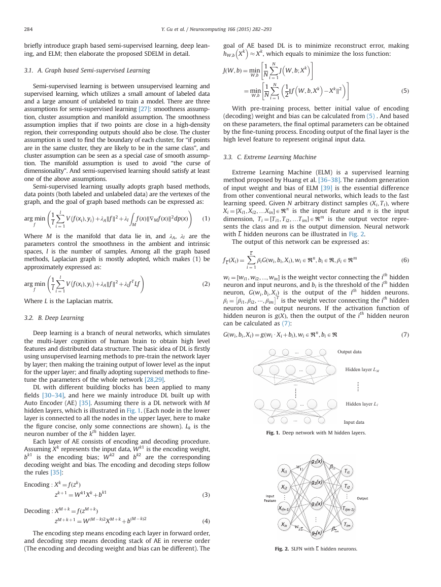DL with different building blocks has been applied to many ﬁelds [30–34], and here we mainly introduce DL built up with Auto Encoder (AE) [35]. Assuming there is a DL network with M hidden layers, which is illustrated in Fig. 1. (Each node in the lower layer is connected to all the nodes in the upper layer, here to make the ﬁgure concise, only some connections are shown). Lk is the neuron number of the kth hidden layer. Each layer of AE consists of encoding and decoding procedure. Assuming Xk represents the input data, W k1 is the encoding weight, bk1 is the encoding bias; W k2 and bk2 are the corresponding decoding weight and bias. The encoding and decoding steps follow the rules [35]: Encoding : Xk ¼ fðzkÞ zkþ 1 ¼ W k1Xk þbk1 ð3Þ Decoding : XM þ k ¼ fðzM þ kÞ zM þ kþ 1 ¼ W M k ð Þ2 Þ2XM þ kþb M k ð4Þ The encoding step means encoding each layer in forward order, and decoding step means decoding stack of AE in reverse order (The encoding and decoding weight and bias can be different). The ð J W; b; Xk ‖f W; b; Xk # Xk‖2 ð5Þ With pre-training process, better initial value of encoding (decoding) weight and bias can be calculated from (5) . And based on these parameters, the ﬁnal optimal parameters can be obtained by the ﬁne-tuning process. Encoding output of the ﬁnal layer is the high level feature to represent original input data. 3.3. C. Extreme Learning Machine Extreme Learning Machine (ELM) is a supervised learning method proposed by Huang et al. [36–38]. The random generation of input weight and bias of ELM [39] is the essential difference from other conventional neural networks, which leads to the fast Þ, where learning speed. 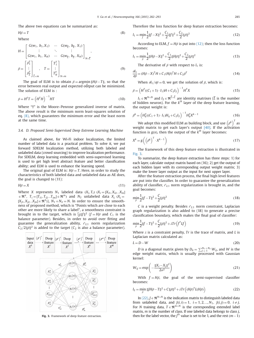Given N arbitrary distinct samples Xi; T i Aℜn is the input feature and n is the input Xi ¼ Xi1; Xi2; …Xin Aℜm is the output vector repre- ½ dimension, T i ¼ T i1; T i2; …T im sents the class and m is the output dimension. Neural network with L hidden neurons can be illustrated in Fig. 2. ð ½ The output of this network can be expressed as: i ¼ 1 ð6Þ βiGðwi; bi; XiÞ; wi Aℜn; bi Aℜ; βi Aℜm ðXiÞ ¼ f L ½ is the weight vector connecting the ith hidden wi ¼ wi1; wi2; :::; win neuron and input neurons, and bi is the threshold of the ith hidden neuron, Gðwi; bi; XiÞ is the output of the ith hidden neurons. βi ¼ βi1; βi2; ⋯; βim neuron and the output neurons. If the activation function of hidden neuron is g Xð Þ, then the output of the ith hidden neuron can be calculated as (7): Gðwi; bi; XiÞ ¼ gðwi UXi þbiÞ; wi Aℜn; bi Aℜ T is the weight vector connecting the ith hidden ð7Þ XL ... ... ... ... ... Output data Hidden layer LM Hidden layer L1 Input data Fig. 1. Deep network with M hidden layers. w w n L Lm L Fig. 2. SLFN with L hidden neurons.

Y. Gu et al. / Neurocomputing 166 (2015) 282–293 285 The above two equations can be summarized as: Hβ ¼ T 2 Where 64 H ¼ 2 664 Gðw1; b1; X1Þ ⋯ GðwL 3 Gðw1; b1; XNÞ ⋯ GðwL 775 βT 1 ⋮ βT L ; bL ⋮ ; bL T T 1 ⋮ T T N ; XNÞ ; X1Þ 2 664 3 775 3 75 T ¼ β ¼ NL ⋱ ⋮ ; ; Nm Lm ð8Þ ð9Þ The goal of ELM is to obtain β ¼ argmin ‖HβT‖, so that the error between real output and expected output can be minimized. The solution of ELM is : β ¼ H†T ¼ HTH 1 ð10Þ HT β Where “†” is the Moore–Penrose generalized inverse of matrix. The above result is the minimum norm least-squares solution of eq. (8), which guarantees the minimum error and the least norm at the same time. 3.4. D. Proposed Semi-Supervised Deep Extreme Learning Machine for Wi-Fi As claimed above, indoor localization, the limited number of labeled data is a practical problem. To solve it, we put forward SDELM localization method, utilizing both labeled and unlabeled data (crowd sourcing) to improve localization performance. For SDELM, deep learning embedded with semi-supervised learning is used to get high level abstract feature and better classiﬁcation ability; and ELM is used to enhance the learning speed. The original goal of ELM is: Hβ ¼ T. Here, in order to study the characteristics of both labeled data and unlabeled data as AE does, the goal is changed to (11): ð11Þ Hβ ¼ X Þ ðXi ¼ ½Xi1; Xi2:::Xin Where X represents N1 labeled data Xi; T i Aℜn; T i ¼ ½T i1; T i2:::T imAℜmÞ and N2 unlabeled data Xj ðXj ¼ ½Xj1; Xj2:::XjnAℜnÞ), N1 þN2 ¼ N. In order to ensure the smooth- ness of proposed method, which is “Points which are close to each other are more likely to share a label”, a smoothness constraint is ‖f ‖2 (f ¼ Hβ and C1 is the brought in to the target, which is C1 2 balance parameter). Besides, in order to avoid over ﬁtting and guarantee the generalization ability, ℓ2;1 norm regularization C2=2‖β‖2 is added to the target (C2 is also a balance parameter). ð Fig. 3. Framework of deep feature extraction. ð13Þ ð14Þ Therefore the loss function for deep feature extraction becomes: l1 ¼ min ð12Þ According to ELM, f ¼ Hβ is put into (12); then the loss function ‖f X‖2 þC1 2 ‖f ‖2 þC2 2 ‖β‖2 1 2 f becomes: 1 l1 ¼ min 2 β ‖HβX‖2 þC1 2 ‖Hβ‖2 þC2 2 ‖β‖2 ∂l1 ∂β ð ÞT HþC1 Hβð The derivative of β with respect to l1 is: ¼ HβX When ∂l1=∂β ¼ 0, we get the solution of β, which is: ÞT HþC2βT 1 ð ð HT X ÞUI1 ÞHþC2I2 β ¼ HT C1 þ1 ð15Þ I1 AℜNN and I2 AℜLL are identity matrixes (L is the number of hidden neuron). For the kth layer of the deep feature learning, the output weight is: βk ¼ HT ÞUI1 ÞHkþC2I2 1 k C1 þ1 ð ð kXk 1 HT T ð16Þ We adopt this modiﬁed ELM as building block, and use βk as weight matrix to get each layer's output [40]. If the activation function is g xð Þ, then the output of the kth layer becomes: Xk ¼ g T UXk 1 ð17Þ βk The framework of this deep feature extraction is illustrated in Fig. 3. To summarize, the deep feature extraction has three steps: 1) for each layer, calculate output matrix based on (16); 2) get the output of each hidden layer with its corresponding output weight matrix; 3) make the lower layer output as the input for next upper layer. After the feature extraction process, the ﬁnal high level features are put into the classiﬁer. In order to guarantee the generalization ability of classiﬁer, ℓ2;1 norm regularization is brought in, and the goal becomes: β min ‖β‖2 ‖f T‖2 þC 2 1 2 C is a weight penalty. Besides ℓ2;1 norm constraint, Laplacian graph regularization is also added to (18) to generate a precise classiﬁcation boundary, which makes the ﬁnal goal of classiﬁer: ð19Þ ‖β‖2 þλTr f T Lf ð18Þ min 1 2 ‖f T‖2 þC 2 β Where λ is a constraint penalty, Tr is the trace of matrix, and L is Laplacian matrix calculated as: L ¼ DW D is a diagonal matrix given by Dii ¼ PN1 þ N2 ð20Þ i ¼ 1 W ij, and W is the edge weight matrix, which is usually processed with Gaussian kernel: ð21Þ ! W ij ¼ exp ‖XiXj‖2 2σ2 With f ¼ Hβ, becomes: l2 ¼ min the goal of the semi-supervised classiﬁer β Þ ÞT L Hβð ‖JHβT‖2 þC‖β‖2 þλTr Hβð ð22Þ In (22), J AℜNN is the indication matrix to distinguish labeled data iaj. from unlabeled data, and J i; i For N training data, T AℜmN is the corresponding extended label matrix, m is the number of class. If one labeled data belongs to class j, then for the label vector, the jth value is set to be 1, and the rest m1 Þ i ¼ 1; 2; :::; N1; Þ ¼ 1; Þ ¼ 0; ð J i; j ð ð

286 Y. Gu et al. / Neurocomputing 166 (2015) 282–293 values become 1; the label vectors for unlabeled data are all set to be 0. In order to get the solution of this optimization problem, we get the derivative of β with respect to l2 in (22), which is: ∂l2 ∂β ¼ JHβT ð23Þ The solution of β satisﬁes the condition that ∂l2=∂β ¼ 0, which h ÞT JHþCβT þλ Hβð ÞT LH ð i 1 ð24Þ is: β ¼ C UIþHT JþλL ð ÞH HT JT Eqs. (16) and (24) are the solutions of weight matrix, which construct the structure of SDELM. Constraint parameters in those equations and the depth of deep feature learning affect the overall performance of SDELM; hence we need to tune these parameters. There are mainly four kinds of parameters in SDELM needed to be tuned, which are weight C1, C2 in deep learning procedure, and weight λ, C in classiﬁer. Usually, cross validation is used to adjust these four parameters. However if the parameters are tuned simultaneously, the time complexity will be Oðn4Þ, which is time- consuming. Therefore, in order to make the adjustment easier and less costly, we adopt hierarchical adjustment mechanism to tune the parameters, which is similar to sparse coding [34] (For sparse coding, it ﬁrstly optimized sparse coefﬁcients with ﬁxed bases, then tuned the bases with ﬁxed coefﬁcients). The parameters are split into two levels according to their level the ﬁrst function; parameters are the parameters in the classiﬁer, and the second level parameters are the parameters in deep learning. Firstly, we assign empirical values to these parameters, and then tune the ﬁrst level's parameters. After optimizing parameters in the ﬁrst level, we adjust the parameters in the second level. With this hierarchical adjustment mechanism, the time complexity can be decreased. 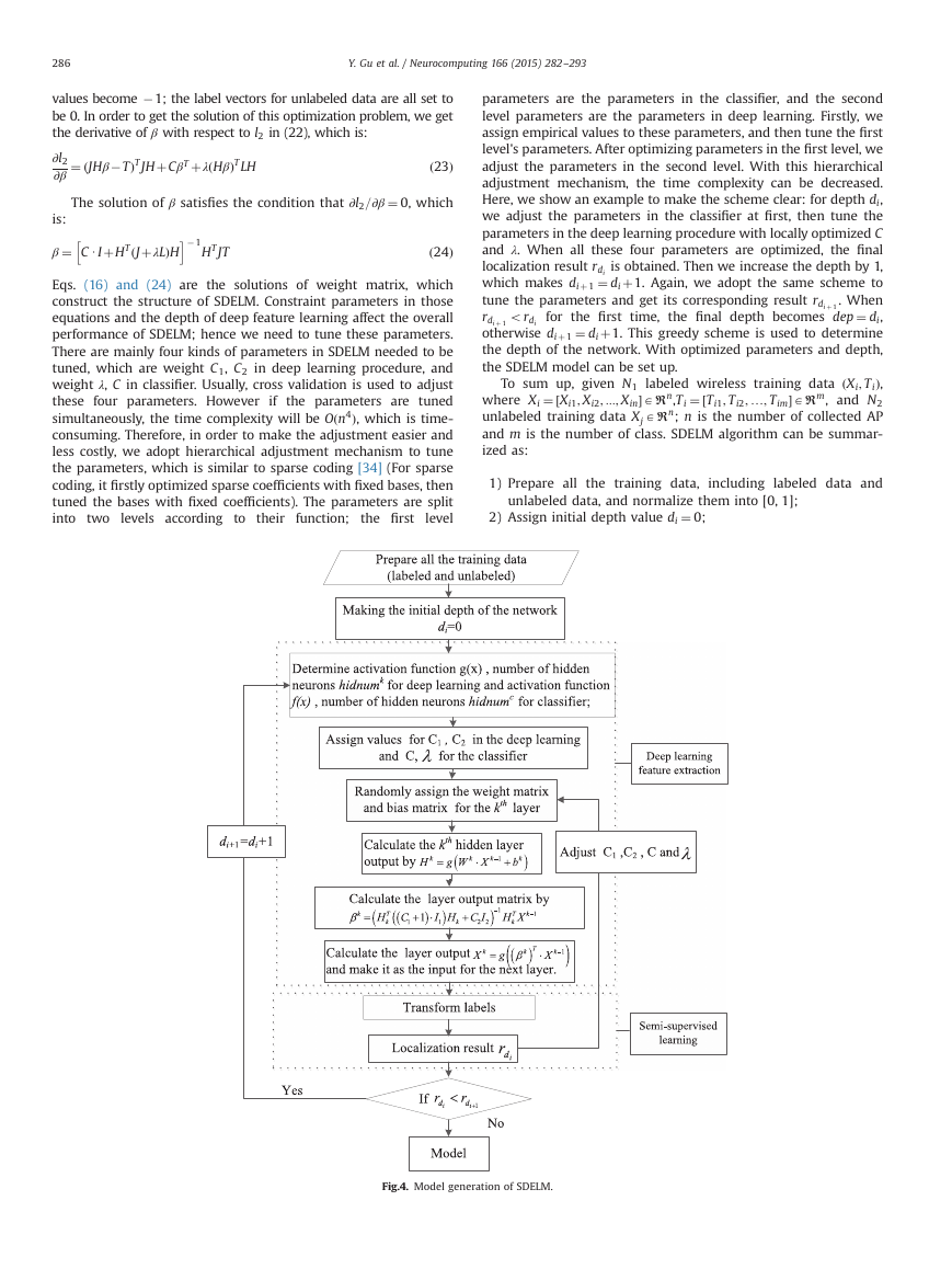Here, we show an example to make the scheme clear: for depth di, we adjust the parameters in the classiﬁer at ﬁrst, then tune the parameters in the deep learning procedure with locally optimized C and λ. When all these four parameters are optimized, the ﬁnal localization result rdi is obtained. Then we increase the depth by 1, which makes diþ 1 ¼ diþ1. Again, we adopt the same scheme to tune the parameters and get its corresponding result rdi þ 1. When for the ﬁrst time, the ﬁnal depth becomes dep ¼ di, rdi þ 1 otherwise diþ 1 ¼ diþ1. This greedy scheme is used to determine the depth of the network. With optimized parameters and depth, the SDELM model can be set up. Þ, To sum up, given N1 labeled wireless training data Xi; T i Aℜm, and N2 where Xi ¼ Xi1; Xi2; :::; Xin unlabeled training data Xj Aℜn; n is the number of collected AP and m is the number of class. SDELM algorithm can be summar- ized as: Aℜn,T i ¼ T i1; T i2; …; T im ordi ð ½ ½ 1) Prepare all the training data, 2) Assign initial depth value di ¼ 0; unlabeled data, and normalize them into [0, 1]; including labeled data and Fig.4. Model generation of SDELM.

Y. Gu et al. / Neurocomputing 166 (2015) 282–293 287 3) Determine activation function g xð Þ, number of hidden neurons hidnumk for deep learning and activation function f xð Þ, num- ber of hidden neurons hidnumc for classiﬁer; 4) Assign initial values for C1, C2 in deep learning and the constrain parameter C, λ in classiﬁer; 5) Randomly assign the weight matrix W k and bias matrix bk for the kth layer; 6) Calculate the kth hidden layer output by equation Hk ¼ g W k UXk 1 þbk 1 layer output matrix by (16): βk ¼ ÞUI1 ; 7) Calculate the kth ÞHk þC2I2 k C1 þ1 ð ð HT kXk 1; HT input for the upper layer; 8) Calculate the output of the kth layer by (17), and make it as the 9) Transform the labels of N1 labeled data to Nnmð 10) Calculate the classiﬁer output weight by (24); 11) Put the last layer output of deep learning into the semi- Þ matrix; supervised classiﬁer to get the result; 12) Utilize hierarchical mechanism to adjust parameters C1, C2, C, and λ, then go through steps 4) to 11) to get the ﬁnal result for the corresponding depth; 13) Make diþ 1 ¼ diþ1, and go through 4) to 12). 14) If rdi þ 1 4rdi , go through 4) to 13), else the model is set up. The model generation framework of proposed SDELM is illu- strated in Fig. 4. 4. Performance Evaluation In this section, performance of proposed SDELM will be validated from four aspects: feature representation, localization accuracy, time consumption and man-hour cost in real indoor environments. 4.1. A. Ofﬁce environment Firstly, localization performance of SDELM is validated in a typical ofﬁce environment. It is a 15 mn10 m area on the 8th ﬂoor of a research building with 24 different locations, whose layout is shown in Fig. 5. Circle points are the locations where labeled data were collected. The reason to choose this environment as test bed is that it is highly dynamic, full of people movement and other changing elements, which can show the complex characteristics of Wi-Fi signal in indoor environment. In this environment, we collected 5695 items of data in one month; 500 of them were randomly chosen as testing data and the rest became training data. The experimental conﬁguration is as follows: DELL PC with 32 bit Operation System, 2.00 G RAM, Intel Core2 CPU, and Matlab R2009b. 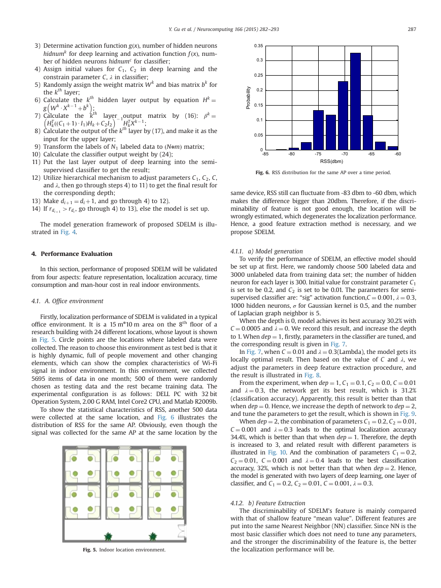To show the statistical characteristics of RSS, another 500 data were collected at the same location, and Fig. 6 illustrates the distribution of RSS for the same AP. Obviously, even though the signal was collected for the same AP at the same location by the Fig. 5. Indoor location environment. 0.35 0.3 0.25 0.2 0.15 0.1 0.05 y t i l i b a b o r P 0 -85 -80 -75 -70 -65 -60 RSS(dbm) Fig. 6. RSS distribution for the same AP over a time period. same device, RSS still can ﬂuctuate from -83 dbm to -60 dbm, which makes the difference bigger than 20dbm. Therefore, if the discri- minability of feature is not good enough, the location will be wrongly estimated, which degenerates the localization performance. Hence, a good feature extraction method is necessary, and we propose SDELM. 4.1.1. a) Model generation To verify the performance of SDELM, an effective model should be set up at ﬁrst. Here, we randomly choose 500 labeled data and 3000 unlabeled data from training data set; the number of hidden neuron for each layer is 300. Initial value for constraint parameter C1 is set to be 0.2, and C2 is set to be 0.01. The parameters for semi- supervised classiﬁer are: “sig” activation function,C ¼ 0:001, λ ¼ 0:3, 1000 hidden neurons, σ for Gaussian kernel is 0.5, and the number of Laplacian graph neighbor is 5. When the depth is 0, model achieves its best accuracy 30.2% with C ¼ 0:0005 and λ ¼ 0. We record this result, and increase the depth to 1. When dep ¼ 1, ﬁrstly, parameters in the classiﬁer are tuned, and the corresponding result is given in Fig. 7. 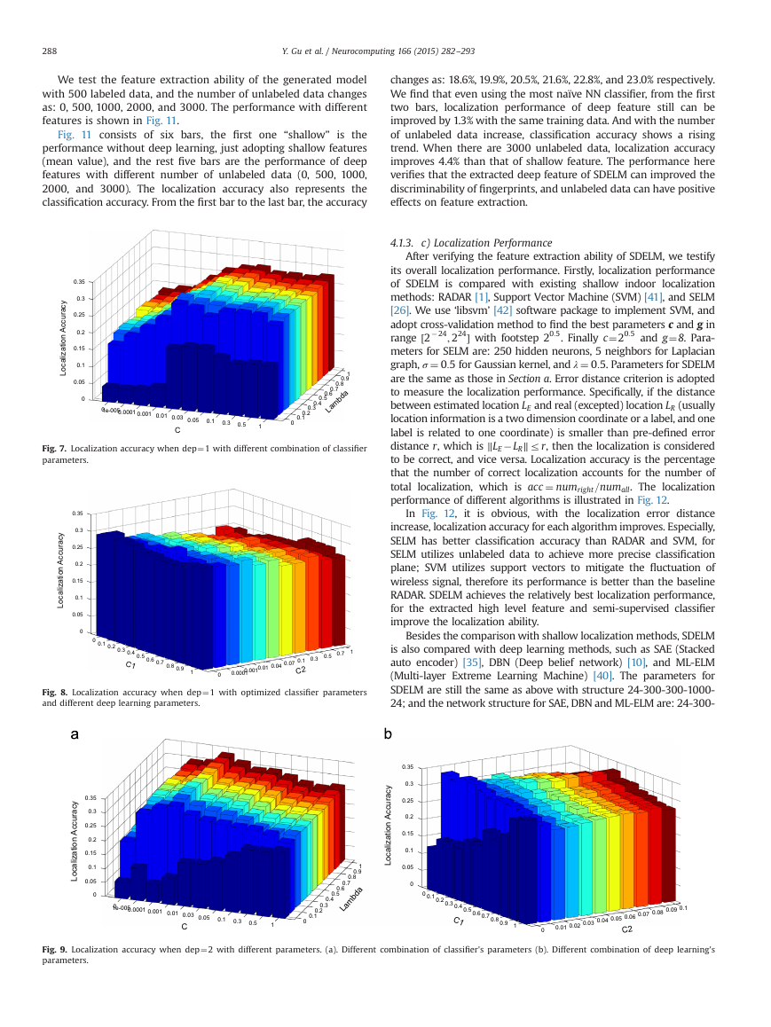In Fig. 7, when C ¼ 0:01 and λ ¼ 0:3(Lambda), the model gets its locally optimal result. Then based on the value of C and λ, we adjust the parameters in deep feature extraction procedure, and the result is illustrated in Fig. 8. From the experiment, when dep ¼ 1, C1 ¼ 0:1, C2 ¼ 0:0, C ¼ 0:01 and λ ¼ 0:3, the network get its best result, which is 31.2% (classiﬁcation accuracy). Apparently, this result is better than that when dep ¼ 0. Hence, we increase the depth of network to dep ¼ 2, and tune the parameters to get the result, which is shown in Fig. 9. When dep ¼ 2, the combination of parameters C1 ¼ 0:2, C2 ¼ 0:01, C ¼ 0:001 and λ ¼ 0:3 leads to the optimal localization accuracy 34.4%, which is better than that when dep ¼ 1. Therefore, the depth is increased to 3, and related result with different parameters is illustrated in Fig. 10. And the combination of parameters C1 ¼ 0:2, C2 ¼ 0:01, C ¼ 0:001 and λ ¼ 0:4 leads to the best classiﬁcation accuracy, 32%, which is not better than that when dep ¼ 2. Hence, the model is generated with two layers of deep learning, one layer of classiﬁer, and C1 ¼ 0:2, C2 ¼ 0:01, C ¼ 0:001, λ ¼ 0:3. 4.1.2. b) Feature Extraction The discriminability of SDELM's feature is mainly compared with that of shallow feature “mean value”. Different features are put into the same Nearest Neighbor (NN) classiﬁer. Since NN is the most basic classiﬁer which does not need to tune any parameters, and the stronger the discriminability of the feature is, the better the localization performance will be.

288 Y. Gu et al. / Neurocomputing 166 (2015) 282–293 We test the feature extraction ability of the generated model with 500 labeled data, and the number of unlabeled data changes as: 0, 500, 1000, 2000, and 3000. The performance with different features is shown in Fig. 11. Fig. 11 consists of six bars, the ﬁrst one “shallow” is the performance without deep learning, just adopting shallow features (mean value), and the rest ﬁve bars are the performance of deep features with different number of unlabeled data (0, 500, 1000, 2000, and 3000). The localization accuracy also represents the classiﬁcation accuracy. From the ﬁrst bar to the last bar, the accuracy changes as: 18.6%, 19.9%, 20.5%, 21.6%, 22.8%, and 23.0% respectively. We ﬁnd that even using the most naïve NN classiﬁer, from the ﬁrst two bars, localization performance of deep feature still can be improved by 1.3% with the same training data. And with the number of unlabeled data increase, classiﬁcation accuracy shows a rising trend. When there are 3000 unlabeled data, localization accuracy improves 4.4% than that of shallow feature. The performance here veriﬁes that the extracted deep feature of SDELM can improved the discriminability of ﬁngerprints, and unlabeled data can have positive effects on feature extraction. y c a r u c c A n o i t a z i l a c o L 0.35 0.3 0.25 0.2 0.15 0.1 0.05 0 01e-0050.0001 0.001 0.01 0.03 0.05 C 0.1 0.3 0.5 1 0 1 0.9 0.8 0.7 0.6 Lambda 0.5 0.4 0.3 0.2 0.1 Fig. 7. Localization accuracy when dep¼1 with different combination of classiﬁer parameters. y c a r u c c A n o i t a z i l a c o L 0.35 0.3 0.25 0.2 0.15 0.1 0.05 0 0 0.1 0.2 0.3 0.4 0.5 0.6 0.7 0.8 0.9 C1 0.00010.0010.01 0.04 0.07 0.1 0.3 0.5 0.7 1 Fig. 8. Localization accuracy when dep¼1 with optimized classiﬁer parameters and different deep learning parameters. C 2 0 1 y c a r u c c A n o i t a z i l a c o L 0.35 0.3 0.25 0.2 0.15 0.1 0.05 0 01e-0050.0001 0.001 0.01 0.03 0.05 C 0.1 0.3 0.5 1 0 1 0.9 0.8 0.5 0.4 0.7 0.6 Lambda 0.3 0.2 0.1 4.1.3. c) Localization Performance After verifying the feature extraction ability of SDELM, we testify its overall localization performance. Firstly, localization performance of SDELM is compared with existing shallow indoor localization methods: RADAR [1], Support Vector Machine (SVM) [41], and SELM [26]. We use ‘libsvm’ [42] software package to implement SVM, and adopt cross-validation method to ﬁnd the best parameters c and g in range ½2 24; 224 with footstep 20:5. Finally c¼20:5 and g¼8. Para- meters for SELM are: 250 hidden neurons, 5 neighbors for Laplacian graph, σ ¼ 0:5 for Gaussian kernel, and λ ¼ 0:5. Parameters for SDELM are the same as those in Section a. Error distance criterion is adopted to measure the localization performance. Speciﬁcally, if the distance between estimated location LE and real (excepted) location LR (usually location information is a two dimension coordinate or a label, and one label is related to one coordinate) is smaller than pre-deﬁned error distance r, which is ‖LE LR‖rr, then the localization is considered to be correct, and vice versa. Localization accuracy is the percentage that the number of correct localization accounts for the number of total localization, which is acc ¼ numright=numall. The localization performance of different algorithms is illustrated in Fig. 12. In Fig. 12, it is obvious, with the localization error distance increase, localization accuracy for each algorithm improves. Especially, SELM has better classiﬁcation accuracy than RADAR and SVM, for SELM utilizes unlabeled data to achieve more precise classiﬁcation plane; SVM utilizes support vectors to mitigate the ﬂuctuation of wireless signal, therefore its performance is better than the baseline RADAR. SDELM achieves the relatively best localization performance, for the extracted high level feature and semi-supervised classiﬁer improve the localization ability. Besides the comparison with shallow localization methods, SDELM is also compared with deep learning methods, such as SAE (Stacked auto encoder) [35], DBN (Deep belief network) [10], and ML-ELM (Multi-layer Extreme Learning Machine) [40]. The parameters for SDELM are still the same as above with structure 24-300-300-1000- 24; and the network structure for SAE, DBN and ML-ELM are: 24-300- y c a r u c c A n o i t a z i l a c o L 0.35 0.3 0.25 0.2 0.15 0.1 0.05 0 0 0.1 0.2 0.3 0.4 0.5 0.6 0.7 0.8 0.9 1 C1 0.01 0.02 0.03 0.04 0.05 0.06 0.07 0.08 0.09 0.1 C 2 0 Fig. 9. Localization accuracy when dep¼2 with different parameters. (a). Different combination of classiﬁer's parameters (b). Different combination of deep learning's parameters.

Y. Gu et al. / Neurocomputing 166 (2015) 282–293 289 y c a r u c c A n o i t a z i l a c o L 0.35 0.3 0.25 0.2 0.15 0.1 0.05 0 01e-0050.00010.001 0.01 0.03 0.05 0.1 0.3 0.5 C 1 0 1 0.9 0.8 0.7 Lambda 0.6 0.5 0.4 0.3 0.2 0.1 y c a r u c c A n o i t a z i l a c o L 0.35 0.3 0.25 0.2 0.15 0.1 0.05 0 0 0.1 0.2 0.3 0.4 0.5 C1 0.6 0.7 0.01 0.02 0.03 0.04 0.05 0.06 0.07 0.08 0.09 0.1 C 2 0.8 0.9 1 0 Fig. 10. Localization accuracy when dep¼3 with different parameters. (a). Different combination of classiﬁer's parameters (b). Different combination of deep learning's parameters. y c a r u c c A n o i t a z i l a c o L 0.25 0.2 0.15 0.1 0.05 0 Shallow D-0 D-500 D-1000 D-2000 D-3000 Fig. 11. Localization performance with the same 500 labeled data and different number of unlabeled data. y c a r u c c A n o i t a z i l a c o L 1 0.9 0.8 0.7 0.6 0.5 0.4 0.3 0.2 0.1 0 RADAR SVM SELM SDELM 1 2 3 4 5 6 7 8 9 10 Error Distance(m) Fig. 12. Localization performance for different localization methods. 24; 24-200-24; 24-500-2000-24 respectively. The localization perfor- mance is shown is Table 1. Form Table 1, we can see that except SDELM, other deep learning methods have similar localization performance, which is better than Table 1 Localization performance for deep learning methods. SAE DBN ML-ELM SDELM Accuracy (%) Training time (s) 29.80 110.3083 31.20 93.3978 29.60 36.8318 34.40 63.9448 shallow localization methods. And SDELM slightly outperforms the other three methods, because it not only extracts high level features as deep learning methods do, but also utilizes semi-supervised classiﬁer to improve the classiﬁcation ability. Besides the localization performance, we also compare the learning speed for different deep learning methods. Apparently, SDELM has less amount of training time than SAE and DBN, for SDELM neither has iterative optimization for the pre-training step, nor needs the ﬁne-tuning procedure. In contrast to ML-ELM, SDELM spends more time, as the calculation of Laplacian matrix is time- consuming. However, considering the trade-off between accuracy and time consumption, SDELM is a reasonable choice to solve the indoor localization problems. 4.1.4. d) Man-hour Cost The goal of SDELM is to utilize unlabeled data to improve localization performance, so that the man-hour of gathering labeled data can be reduced. Hence, how much man-hour of calibration can be saved is tested in this part. In Fig. 12, in order to achieve approximately 34% localization accuracy (34.4%) when the error distance is 1 m, 500 labeled data and 3000 unlabeled data are needed. Here, we only use labeled data and change the number of them to get the same localization performance, and the result is shown in Fig. 13. Parameters of SDELM are the same as those in Section c. In Fig. 13, when error distance is 1 m, the localization accuracy changes as: 24.4%, 28.8%, 32.1%, 33.3%, and 35.4% with different number of labeled data. The result indicates that 1500 or 2000 labeled data are needed to achieve approximately 34% (33.3% or 35.4%) localization accuracy when the error distance is 1 m. How- ever, when unlabeled data are used to assist localization, from Fig. 12, we ﬁnd that only 500 labeled data are required to achieve the same localization performance (34.4%), which means with the help of unlabeled data, man-hour can be saved to achieve the same result.

分享到：

赞收藏

资料库

半监督式深度极限学习机，用于基于Wi-Fi的本地化.pdf

相关推荐

开发技术

热门标签

最新资料