4
1
0
2
r
p
A
1
1
]
G
L
.
s
c
[
1
v
6
8
9
2
.
4
0
4
1
:
v
i
X
r
a
A Tutorial on Independent Component Analysis
Jonathon Shlens∗
Google Research
Mountain View, CA 94043
(Dated: April 14, 2014; Version 1.0)
Independent component analysis (ICA) has become a standard data analysis technique applied to an array of
problems in signal processing and machine learning. This tutorial provides an introduction to ICA based on
linear algebra formulating an intuition for ICA from first principles. The goal of this tutorial is to provide a solid
foundation on this advanced topic so that one might learn the motivation behind ICA, learn why and when to
apply this technique and in the process gain an introduction to this exciting field of active research.
I. INTRODUCTION
Measurements often do not reflect the very thing intended to
be measured. Measurements are corrupted by random noise –
but that is only one piece of the story. Often, measurements
can not be made in isolation, but reflect the combination of
many distinct sources. For instance, try to record a person’s
voice on a city street. The faint crackle of the tape can be
heard in the recording but so are the sounds of cars, other
pedestrians, footsteps, etc. Sometimes the main obstacle pre-
venting a clean measurement is not just noise in the traditional
sense (e.g. faint crackle) but independent signals arising from
distinct, identifiable sources (e.g. cars, footsteps).
The distinction is subtle. We could view a measurement as an
estimate of a single source corrupted by some random fluc-
tuations (e.g. additive white noise). Instead, we assert that a
measurement can be a combination of many distinct sources
– each different from random noise. The broad topic of sep-
arating mixed sources has a name - blind source separation
(BSS). As of today’s writing, solving an arbitrary BSS prob-
lem is often intractable. However, a small subset of these
types of problem have been solved only as recently as the last
two decades – this is the provenance of independent compo-
nent analysis (ICA).
Solving blind source separation using ICA has two related in-
terpretations – filtering and dimensional reduction.
If each
source can be identified, a practitioner might choose to selec-
tively delete or retain a single source (e.g. a person’s voice,
above). This is a filtering operation in the sense that some
aspect of the data is selectively removed or retained. A filter-
ing operation is equivalent to projecting out some aspect (or
dimension) of the data – in other words a prescription for di-
mensional reduction. Filtering data based on ICA has found
many applications including the analysis of photographic im-
ages, medical signals (e.g. EEG, MEG, MRI, etc.), biological
assays (e.g. micro-arrays, gene chips, etc.) and most notably
audio signal processing.
∗Electronic address: jonathon.shlens@gmail.com
ICA can be applied to data in a naive manner treating the tech-
nique as a sophisticated black box that essentially performs
“magic”. While empowering, deploying a technique in this
manner is fraught with peril. For instance, how does one judge
the success of ICA? When will ICA fail? When are other
methods more appropriate? I believe that understanding these
questions and the method itself are necessary for appreciating
when and how to apply ICA. It is for these reasons that I write
this tutorial.
This tutorial is not a scholarly paper. Nor is it thorough.
The goal of this paper is simply to educate. That said, the
ideas in this tutorial are sophisticated.
I presume that the
reader is comfortable with linear algebra, basic probability
and statistics as well as the topic of principal component anal-
ysis (PCA).1 This paper does not shy away from informal ex-
planations but also stresses the mathematics when they shed
insight on to the problem. As always, please feel free to email
me with any comments, concerns or corrections.2
II. MEASUREMENTS IN THE REAL WORLD
While the mathematics underlying the problems of blind
source separation (BSS) are formidable, the ideas underlying
BSS are quite intuitive. This section focuses on building this
intuition by asking how signals interact in the real world when
we make a measurement in which multiple sources contribute
in addition to noise.
Many experiments have domain-specific knowledge behind
how a measurement is performed.
(How does a gene chip
work?) Instead, this tutorial describes how measurements are
made in domains in which we are all experts – our own senses.
1 A good introduction to PCA written in the same style is A Tutorial on
Principal Component Analysis by yours truly. This tutorial provides a full
introduction and discussion of PCA with concrete examples for building
intuition.
2 I wish to offer a special thanks to E. Simoncelli for many fruitful discus-
sions and insights and U. Rajashekar for thoughtful discussion, editing and
feedback.
�
We discuss what a BSS problem entails in the visual and audi-
tory domains and in the process build some intuition for what
it takes to solve such a problem.
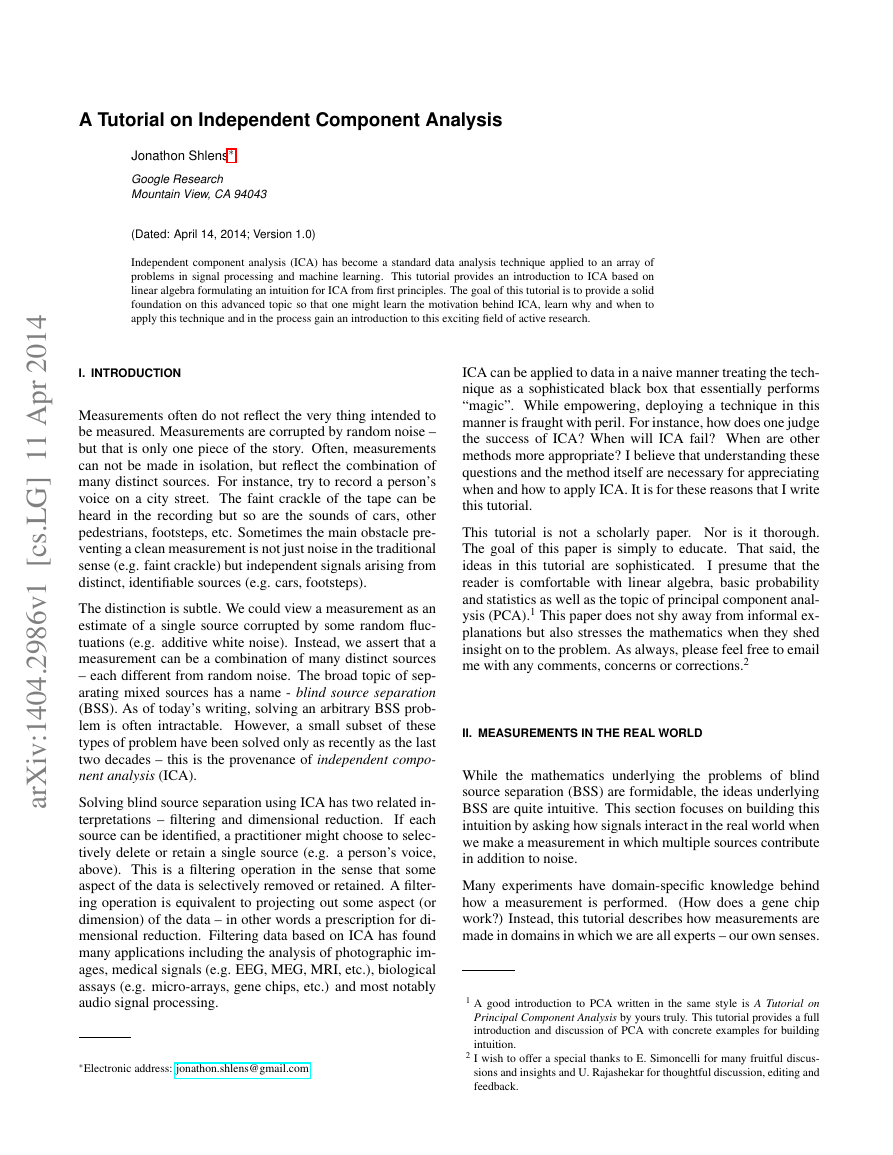
No better example exists of a BSS problem than sound. A
fundamental observation from physics is that sound adds lin-
early. Whatever is recorded in a microphone or registered in
our ear drum is the sum of the pressure waves from emanat-
ing from multiple sources. Consider an everyday problem.
Amongst a background of music and conversations, we must
discern a single person’s voice. The cocktail party problem is
a classic problem in auditory signal processing. The goal of
the cocktail party problem is to discern the sound associated
with a single object even though all of the sounds in the envi-
ronment are superimposed on one another (Figure 1). This is a
challenging and highly applicable problem that only in recent
years have reasonable solutions been devised based on ideas
from ICA.
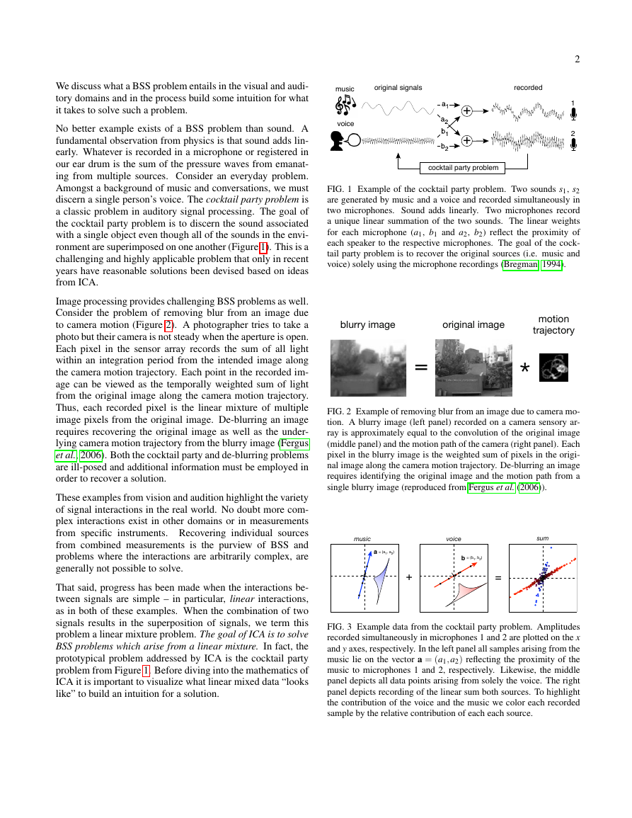
Image processing provides challenging BSS problems as well.
Consider the problem of removing blur from an image due
to camera motion (Figure 2). A photographer tries to take a
photo but their camera is not steady when the aperture is open.
Each pixel in the sensor array records the sum of all light
within an integration period from the intended image along
the camera motion trajectory. Each point in the recorded im-
age can be viewed as the temporally weighted sum of light
from the original image along the camera motion trajectory.
Thus, each recorded pixel is the linear mixture of multiple
image pixels from the original image. De-blurring an image
requires recovering the original image as well as the under-
lying camera motion trajectory from the blurry image (Fergus
et al., 2006). Both the cocktail party and de-blurring problems
are ill-posed and additional information must be employed in
order to recover a solution.
These examples from vision and audition highlight the variety
of signal interactions in the real world. No doubt more com-
plex interactions exist in other domains or in measurements
from specific instruments. Recovering individual sources
from combined measurements is the purview of BSS and
problems where the interactions are arbitrarily complex, are
generally not possible to solve.
That said, progress has been made when the interactions be-
tween signals are simple – in particular, linear interactions,
as in both of these examples. When the combination of two
signals results in the superposition of signals, we term this
problem a linear mixture problem. The goal of ICA is to solve
BSS problems which arise from a linear mixture. In fact, the
prototypical problem addressed by ICA is the cocktail party
problem from Figure 1. Before diving into the mathematics of
ICA it is important to visualize what linear mixed data “looks
like” to build an intuition for a solution.
2
FIG. 1 Example of the cocktail party problem. Two sounds s1, s2
are generated by music and a voice and recorded simultaneously in
two microphones. Sound adds linearly. Two microphones record
a unique linear summation of the two sounds. The linear weights
for each microphone (a1, b1 and a2, b2) reflect the proximity of
each speaker to the respective microphones. The goal of the cock-
tail party problem is to recover the original sources (i.e. music and
voice) solely using the microphone recordings (Bregman, 1994).
FIG. 2 Example of removing blur from an image due to camera mo-
tion. A blurry image (left panel) recorded on a camera sensory ar-
ray is approximately equal to the convolution of the original image
(middle panel) and the motion path of the camera (right panel). Each
pixel in the blurry image is the weighted sum of pixels in the origi-
nal image along the camera motion trajectory. De-blurring an image
requires identifying the original image and the motion path from a
single blurry image (reproduced from Fergus et al. (2006)).
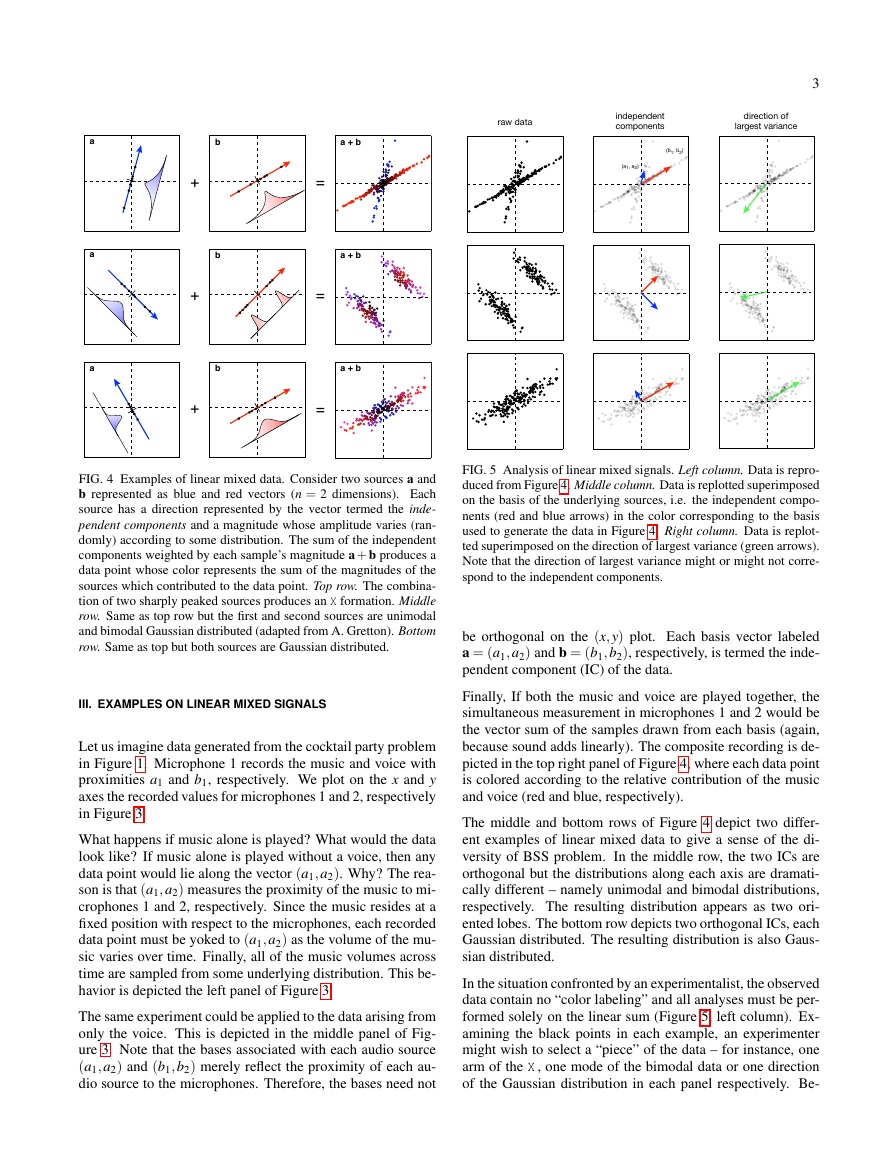
FIG. 3 Example data from the cocktail party problem. Amplitudes
recorded simultaneously in microphones 1 and 2 are plotted on the x
and y axes, respectively. In the left panel all samples arising from the
music lie on the vector a = (a1,a2) reflecting the proximity of the
music to microphones 1 and 2, respectively. Likewise, the middle
panel depicts all data points arising from solely the voice. The right
panel depicts recording of the linear sum both sources. To highlight
the contribution of the voice and the music we color each recorded
sample by the relative contribution of each each source.
recordedoriginal signalsmusicvoicecocktail party problem++12∗=blurry imageoriginal imagemotion
trajectory+=musicvoicesum= (b1, b2)= (a1, a2)ab�
3
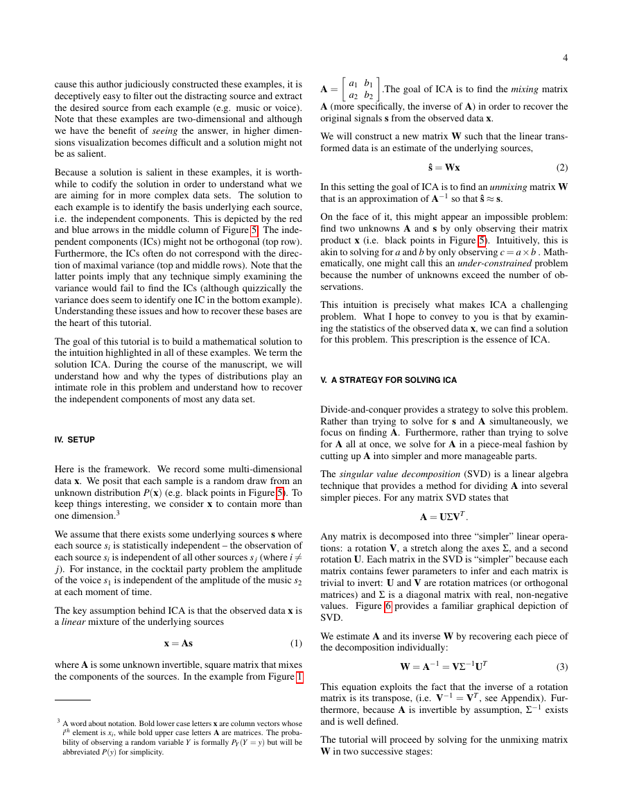
FIG. 4 Examples of linear mixed data. Consider two sources a and
b represented as blue and red vectors (n = 2 dimensions). Each
source has a direction represented by the vector termed the inde-
pendent components and a magnitude whose amplitude varies (ran-
domly) according to some distribution. The sum of the independent
components weighted by each sample’s magnitude a + b produces a
data point whose color represents the sum of the magnitudes of the
sources which contributed to the data point. Top row. The combina-
tion of two sharply peaked sources produces an X formation. Middle
row. Same as top row but the first and second sources are unimodal
and bimodal Gaussian distributed (adapted from A. Gretton). Bottom
row. Same as top but both sources are Gaussian distributed.
III. EXAMPLES ON LINEAR MIXED SIGNALS
Let us imagine data generated from the cocktail party problem
in Figure 1. Microphone 1 records the music and voice with
proximities a1 and b1, respectively. We plot on the x and y
axes the recorded values for microphones 1 and 2, respectively
in Figure 3.
What happens if music alone is played? What would the data
look like? If music alone is played without a voice, then any
data point would lie along the vector (a1,a2). Why? The rea-
son is that (a1,a2) measures the proximity of the music to mi-
crophones 1 and 2, respectively. Since the music resides at a
fixed position with respect to the microphones, each recorded
data point must be yoked to (a1,a2) as the volume of the mu-
sic varies over time. Finally, all of the music volumes across
time are sampled from some underlying distribution. This be-
havior is depicted the left panel of Figure 3.
The same experiment could be applied to the data arising from
only the voice. This is depicted in the middle panel of Fig-
ure 3. Note that the bases associated with each audio source
(a1,a2) and (b1,b2) merely reflect the proximity of each au-
dio source to the microphones. Therefore, the bases need not
FIG. 5 Analysis of linear mixed signals. Left column. Data is repro-
duced from Figure 4. Middle column. Data is replotted superimposed
on the basis of the underlying sources, i.e. the independent compo-
nents (red and blue arrows) in the color corresponding to the basis
used to generate the data in Figure 4. Right column. Data is replot-
ted superimposed on the direction of largest variance (green arrows).
Note that the direction of largest variance might or might not corre-
spond to the independent components.
be orthogonal on the (x,y) plot. Each basis vector labeled
a = (a1,a2) and b = (b1,b2), respectively, is termed the inde-
pendent component (IC) of the data.
Finally, If both the music and voice are played together, the
simultaneous measurement in microphones 1 and 2 would be
the vector sum of the samples drawn from each basis (again,
because sound adds linearly). The composite recording is de-
picted in the top right panel of Figure 4, where each data point
is colored according to the relative contribution of the music
and voice (red and blue, respectively).
The middle and bottom rows of Figure 4 depict two differ-
ent examples of linear mixed data to give a sense of the di-
versity of BSS problem. In the middle row, the two ICs are
orthogonal but the distributions along each axis are dramati-
cally different – namely unimodal and bimodal distributions,
respectively. The resulting distribution appears as two ori-
ented lobes. The bottom row depicts two orthogonal ICs, each
Gaussian distributed. The resulting distribution is also Gaus-
sian distributed.
In the situation confronted by an experimentalist, the observed
data contain no “color labeling” and all analyses must be per-
formed solely on the linear sum (Figure 5, left column). Ex-
amining the black points in each example, an experimenter
might wish to select a “piece” of the data – for instance, one
arm of the X , one mode of the bimodal data or one direction
of the Gaussian distribution in each panel respectively. Be-
+=b+=aba + b+=aa + bindependent
componentsa + babraw dataindependent
componentsdirection of
largest variance(b1, b2)(a1, a2)�
cause this author judiciously constructed these examples, it is
deceptively easy to filter out the distracting source and extract
the desired source from each example (e.g. music or voice).
Note that these examples are two-dimensional and although
we have the benefit of seeing the answer, in higher dimen-
sions visualization becomes difficult and a solution might not
be as salient.
Because a solution is salient in these examples, it is worth-
while to codify the solution in order to understand what we
are aiming for in more complex data sets. The solution to
each example is to identify the basis underlying each source,
i.e. the independent components. This is depicted by the red
and blue arrows in the middle column of Figure 5. The inde-
pendent components (ICs) might not be orthogonal (top row).
Furthermore, the ICs often do not correspond with the direc-
tion of maximal variance (top and middle rows). Note that the
latter points imply that any technique simply examining the
variance would fail to find the ICs (although quizzically the
variance does seem to identify one IC in the bottom example).
Understanding these issues and how to recover these bases are
the heart of this tutorial.
The goal of this tutorial is to build a mathematical solution to
the intuition highlighted in all of these examples. We term the
solution ICA. During the course of the manuscript, we will
understand how and why the types of distributions play an
intimate role in this problem and understand how to recover
the independent components of most any data set.
IV. SETUP
Here is the framework. We record some multi-dimensional
data x. We posit that each sample is a random draw from an
unknown distribution P(x) (e.g. black points in Figure 5). To
keep things interesting, we consider x to contain more than
one dimension.3
We assume that there exists some underlying sources s where
each source si is statistically independent – the observation of
each source si is independent of all other sources s j (where i =
j). For instance, in the cocktail party problem the amplitude
of the voice s1 is independent of the amplitude of the music s2
at each moment of time.
The key assumption behind ICA is that the observed data x is
a linear mixture of the underlying sources
x = As
(1)
where A is some unknown invertible, square matrix that mixes
the components of the sources. In the example from Figure 1
3 A word about notation. Bold lower case letters x are column vectors whose
ith element is xi, while bold upper case letters A are matrices. The proba-
bility of observing a random variable Y is formally PY (Y = y) but will be
abbreviated P(y) for simplicity.
a1 b1
4
a2 b2
A =
.The goal of ICA is to find the mixing matrix
A (more specifically, the inverse of A) in order to recover the
original signals s from the observed data x.
We will construct a new matrix W such that the linear trans-
formed data is an estimate of the underlying sources,
ˆs = Wx
(2)
In this setting the goal of ICA is to find an unmixing matrix W
that is an approximation of A−1 so that ˆs ≈ s.
On the face of it, this might appear an impossible problem:
find two unknowns A and s by only observing their matrix
product x (i.e. black points in Figure 5). Intuitively, this is
akin to solving for a and b by only observing c = a×b . Math-
ematically, one might call this an under-constrained problem
because the number of unknowns exceed the number of ob-
servations.
This intuition is precisely what makes ICA a challenging
problem. What I hope to convey to you is that by examin-
ing the statistics of the observed data x, we can find a solution
for this problem. This prescription is the essence of ICA.
V. A STRATEGY FOR SOLVING ICA
Divide-and-conquer provides a strategy to solve this problem.
Rather than trying to solve for s and A simultaneously, we
focus on finding A. Furthermore, rather than trying to solve
for A all at once, we solve for A in a piece-meal fashion by
cutting up A into simpler and more manageable parts.
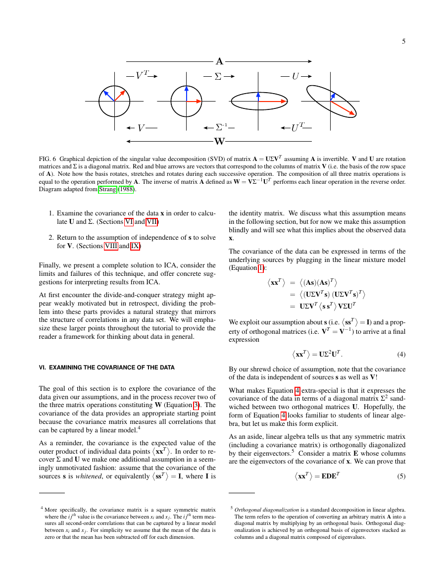
The singular value decomposition (SVD) is a linear algebra
technique that provides a method for dividing A into several
simpler pieces. For any matrix SVD states that
A = UΣVT .
Any matrix is decomposed into three “simpler” linear opera-
tions: a rotation V, a stretch along the axes Σ, and a second
rotation U. Each matrix in the SVD is “simpler” because each
matrix contains fewer parameters to infer and each matrix is
trivial to invert: U and V are rotation matrices (or orthogonal
matrices) and Σ is a diagonal matrix with real, non-negative
values. Figure 6 provides a familiar graphical depiction of
SVD.
We estimate A and its inverse W by recovering each piece of
the decomposition individually:
W = A−1 = VΣ−1UT
(3)
This equation exploits the fact that the inverse of a rotation
matrix is its transpose, (i.e. V−1 = VT , see Appendix). Fur-
thermore, because A is invertible by assumption, Σ−1 exists
and is well defined.
The tutorial will proceed by solving for the unmixing matrix
W in two successive stages:
�
5
FIG. 6 Graphical depiction of the singular value decomposition (SVD) of matrix A = UΣVT assuming A is invertible. V and U are rotation
matrices and Σ is a diagonal matrix. Red and blue arrows are vectors that correspond to the columns of matrix V (i.e. the basis of the row space
of A). Note how the basis rotates, stretches and rotates during each successive operation. The composition of all three matrix operations is
equal to the operation performed by A. The inverse of matrix A defined as W = VΣ−1UT performs each linear operation in the reverse order.
Diagram adapted from Strang (1988).
1. Examine the covariance of the data x in order to calcu-
late U and Σ. (Sections VI and VII)
2. Return to the assumption of independence of s to solve
for V. (Sections VIII and IX)
Finally, we present a complete solution to ICA, consider the
limits and failures of this technique, and offer concrete sug-
gestions for interpreting results from ICA.
At first encounter the divide-and-conquer strategy might ap-
pear weakly motivated but in retrospect, dividing the prob-
lem into these parts provides a natural strategy that mirrors
the structure of correlations in any data set. We will empha-
size these larger points throughout the tutorial to provide the
reader a framework for thinking about data in general.
VI. EXAMINING THE COVARIANCE OF THE DATA
The goal of this section is to explore the covariance of the
data given our assumptions, and in the process recover two of
the three matrix operations constituting W (Equation 3). The
covariance of the data provides an appropriate starting point
because the covariance matrix measures all correlations that
can be captured by a linear model.4
As a reminder, the covariance is the expected value of the
outer product of individual data pointsxxT. In order to re-
sources s is whitened, or equivalentlyssT = I, where I is
cover Σ and U we make one additional assumption in a seem-
ingly unmotivated fashion: assume that the covariance of the
the identity matrix. We discuss what this assumption means
in the following section, but for now we make this assumption
blindly and will see what this implies about the observed data
x.
The covariance of the data can be expressed in terms of the
underlying sources by plugging in the linear mixture model
(Equation 1):xxT = (As)(As)T
We exploit our assumption about s (i.e.ssT = I) and a prop-
= (UΣVT s) (UΣVT s)T
= UΣVTs sTVΣUT
erty of orthogonal matrices (i.e. VT = V−1) to arrive at a final
expression
xxT = UΣ2UT .
By our shrewd choice of assumption, note that the covariance
of the data is independent of sources s as well as V!
What makes Equation 4 extra-special is that it expresses the
covariance of the data in terms of a diagonal matrix Σ2 sand-
wiched between two orthogonal matrices U. Hopefully, the
form of Equation 4 looks familiar to students of linear alge-
bra, but let us make this form explicit.
As an aside, linear algebra tells us that any symmetric matrix
(including a covariance matrix) is orthogonally diagonalized
by their eigenvectors.5 Consider a matrix E whose columns
are the eigenvectors of the covariance of x. We can prove that
xxT = EDET
(4)
(5)
4 More specifically, the covariance matrix is a square symmetric matrix
where the i jth value is the covariance between xi and x j. The i jth term mea-
sures all second-order correlations that can be captured by a linear model
between xi and x j. For simplicity we assume that the mean of the data is
zero or that the mean has been subtracted off for each dimension.
5 Orthogonal diagonalization is a standard decomposition in linear algebra.
The term refers to the operation of converting an arbitrary matrix A into a
diagonal matrix by multiplying by an orthogonal basis. Orthogonal diag-
onalization is achieved by an orthogonal basis of eigenvectors stacked as
columns and a diagonal matrix composed of eigenvalues.
UΣVTAWUTVΣ-1�
where D is a diagonal matrix of associated eigenvalues (see
Appendix). The eigenvectors of the covariance of the data
form an orthonormal basis meaning that E is an orthogonal
matrix.
Compare Equations 4 and 5. Both equations state that the
covariance of the data can be diagonalized by an orthogonal
matrix. Equation 4 provides a decomposition based on the
underlying assumption of ICA. Equation 5 provides a decom-
position based purely on the properties of symmetric matrices.
Diagonalizing a symmetric matrix using its eigenvectors is a
unique solution up to a permutation, i.e. no other basis can
diagonalize a symmetric matrix. Therefore, if our assump-
tions behind ICA are correct, then we have identified a partial
solution to A: U is a matrix of the stacked eigenvectors of
the covariance of the data and Σ is a diagonal matrix with the
square root of the associated eigenvalue in the diagonal.
Let us summarize our current state. We are constructing a
new matrix W via Equation 3. We have identified the latter
two matrices such that
W = VD− 1
2 ET .
D and E are the eigenvalues and eigenvectors of the covari-
ance of the data x. V is the sole unknown rotation matrix. Let
us now take a moment to interpret our results.
VII. WHITENING, REVISITED
The solution for ICA thus far performs an operation famil-
iar to signal processing termed whitening. Whitening is an
operation that removes all linear dependencies in a data set
(i.e. second-order correlations) and normalizes the variance
along all dimensions. Colloquially, this operation is termed
sphereing the data as intuitively, whitening maps the data into
a spherically symmetric distribution.
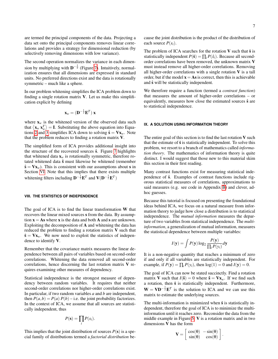
This intuition is demonstrated by the two operations D− 1
2 ET
depicted in Figure 7. In the first step the data is rotated to align
the eigenvectors of the covariance along the cartesian basis.
Multiplying by ET performs this rotation in order to decor-
relate the data, i.e. remove linear dependencies. Mathemat-
ically, decorrelation means that the covariance of the trans-
formed data is diagnolized. In our case,
(ET x) (ET x)T = D
where D is a diagonal matrix of the eigenvalues.6 Each diag-
onal entry in D is an eigenvalue of the covariance of the data
and measures the variance along each dimension.
This operation has a familiar name - principal component
analysis (PCA). The eigenvectors of the covariance of the data
6
FIG. 7 Whitening a data set can be represented as a series of two
linear operations. Data is projected on the principal components,
ET x. Each axis is then scaled so that every direction has unit vari-
ance, D− 1
2 ET x. The red arrow indicates the transformation of the
eigenvector with the largest variance.
from Equation 5,
xxT = EDET
ETxxTE = D
ET xxT E = D
(ET x) (ET x)T = D
6 This equation directly results from orthogonal diagonalization. Starting
We have exploited the property that E is an orthogonal matrix as well as
the linearity of expectations.
D−12decorrelation (PCA)normalizationET�
7
cause the joint distribution is the product of the distribution of
each source P(si).
The problem of ICA searches for the rotation V such that ˆs is
statistically independent P(ˆs) = ∏i P( ˆsi). Because all second-
order correlations have been removed, the unknown matrix V
must instead remove all higher-order correlations. Removing
all higher-order correlations with a single rotation V is a tall
order, but if the model x = As is correct, then this is achievable
and ˆs will be statistically independent.
We therefore require a function (termed a contrast function)
that measures the amount of higher-order correlations – or
equivalently, measures how close the estimated sources ˆs are
to statistical independence.
IX. A SOLUTION USING INFORMATION THEORY
The entire goal of this section is to find the last rotation V such
that the estimate of ˆs is statistically independent. To solve this
problem, we resort to a branch of mathematics called informa-
tion theory. The mathematics of information theory is quite
distinct. I would suggest that those new to this material skim
this section in their first reading.
Many contrast functions exist for measuring statistical inde-
pendence of ˆs. Examples of contrast functions include rig-
orous statistical measures of correlations, approximations to
said measures (e.g. see code in Appendix B) and clever, ad-
hoc guesses.
Because this tutorial is focused on presenting the foundational
ideas behind ICA, we focus on a natural measure from infor-
mation theory to judge how close a distribution is to statistical
independence. The mutual information measures the depar-
ture of two variables from statistical independence. The multi-
information, a generalization of mutual information, measures
the statistical dependence between multiple variables:
I(y) =
P(y)log2
P(y)
∏i P(yi)
dy
are termed the principal components of the data. Projecting a
data set onto the principal components removes linear corre-
lations and provides a strategy for dimensional reduction (by
selectively removing dimensions with low variance).
The second operation normalizes the variance in each dimen-
sion by multiplying with D− 1
2 (Figure 7). Intuitively, normal-
ization ensures that all dimensions are expressed in standard
units. No preferred directions exist and the data is rotationally
symmetric – much like a sphere.
In our problem whitening simplifies the ICA problem down to
finding a single rotation matrix V. Let us make this simplifi-
cation explicit by defining
xw = (D− 1
2 ET ) x
w
where xw is the whitened version of the observed data such
= I. Substituting the above equation into Equa-
thatxw xT
tions 2 and 3 simplifies ICA down to solving ˆs = Vxw. Note
that the problem reduces to finding a rotation matrix V.
The simplified form of ICA provides additional insight into
the structure of the recovered sources ˆs. Figure 7 highlights
that whitened data xw is rotationally symmetric, therefore ro-
tated whitened data ˆs must likewise be whitened (remember
ˆs = Vxw). This is consistent with our assumptions about s in
Section VI. Note that this implies that there exists multiple
whitening filters including D− 1
2 ET and V(D− 1
2 ET )
VIII. THE STATISTICS OF INDEPENDENCE
The goal of ICA is to find the linear transformation W that
recovers the linear mixed sources s from the data. By assump-
tion x = As where x is the data and both A and s are unknown.
Exploiting the decomposition of A and whitening the data has
reduced the problem to finding a rotation matrix V such that
ˆs = Vxw. We now need to exploit the statistics of indepen-
dence to identify V.
Remember that the covariance matrix measures the linear de-
pendence between all pairs of variables based on second-order
correlations. Whitening the data removed all second-order
correlations, hence discerning the last rotation matrix V re-
quires examining other measures of dependency.
Statistical independence is the strongest measure of depen-
dency between random variables.
It requires that neither
second-order correlations nor higher-order correlations exist.
In particular, if two random variables a and b are independent,
then P(a,b) = P(a) P(b) – i.e. the joint probability factorizes.
In the context of ICA, we assume that all sources are statisti-
cally independent, thus
P(s) = ∏
i
P(si).
It is a non-negative quantity that reaches a minimum of zero
if and only if all variables are statistically independent. For
example, if P(y) = ∏i P(yi), then log(1) = 0 and I(y) = 0.
The goal of ICA can now be stated succinctly. Find a rotation
matrix V such that I(ˆs) = 0 where ˆs = Vxw. If we find such
a rotation, then ˆs is statistically independent. Furthermore,
W = VD− 1
2 ET is the solution to ICA and we can use this
matrix to estimate the underlying sources.
The multi-information is minimized when ˆs is statistically in-
dependent, therefore the goal of ICA is to minimize the multi-
information until it reaches zero. Reconsider the data from the
middle example in Figure 5. V is a rotation matrix and in two
dimensions V has the form
cos(θ) −sin(θ)
.
sin(θ)
cos(θ)
This implies that the joint distribution of sources P(s) is a spe-
cial family of distributions termed a factorial distribution be-
V =
�
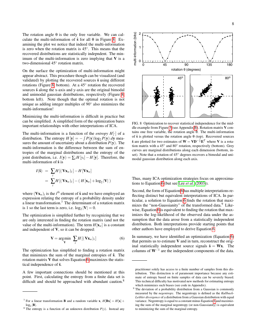
The rotation angle θ is the only free variable. We can cal-
culate the multi-information of ˆs for all θ in Figure 8. Ex-
amining the plot we notice that indeed the multi-information
is zero when the rotation matrix is 45◦. This means that the
recovered distributions are statistically indepndent. The min-
imum of the multi-information is zero implying that V is a
two-dimensional 45◦ rotation matrix.
On the surface the optimization of multi-information might
appear abstract. This procedure though can be visualized (and
validated) by plotting the recovered sources ˆs using different
rotations (Figure 8, bottom). At a 45◦ rotation the recovered
sources ˆs along the x-axis and y-axis are the original bimodal
and unimodal gaussian distributions, respectively (Figure 8,
bottom left). Note though that the optimal rotation is not
unique as adding integer multiples of 90◦ also minimizes the
multi-information!
Minimizing the multi-information is difficult in practice but
can be simplified. A simplified form of the optimization bares
important relationships with other interpretations of ICA.
The multi-information is a function of the entropy H[·] of a
distribution. The entropy H [y] = − P(y)log2 P(y) dy mea-
sures the amount of uncertainty about a distribution P(y). The
multi-information is the difference between the sum of en-
tropies of the marginal distributions and the entropy of the
joint distribution, i.e. I(y) = ∑i H [yi]− H [y]. Therefore, the
multi-information of ˆs is
I(ˆs) = ∑
= ∑
i
i
H [(Vxw)i ]− H [Vxw]
H [(Vxw)i ]− ( H [xw] + log2|V| )
where (Vxw)i is the ith element of ˆs and we have employed an
expression relating the entropy of a probability density under
a linear transformation.7 The determinant of a rotation matrix
is 1 so the last term is zero, i.e. log2|V| = 0.
The optimization is simplified further by recognizing that we
are only interested in finding the rotation matrix (and not the
value of the multi-information). The term H[xw] is a constant
and independent of V, so it can be dropped:
V = argmin
V
∑
i
H [(Vxw)i ]
(6)
The optimization has simplified to finding a rotation matrix
that minimizes the sum of the marginal entropies of ˆs. The
rotation matrix V that solves Equation 6 maximizes the statis-
tical independence of ˆs.
A few important connections should be mentioned at this
point. First, calculating the entropy from a finite data set is
difficult and should be approached with abundant caution.8
7 For a linear transformation B and a random variable x, H[Bx] = H[x] +
log2 |B|.
8 The entropy is a function of an unknown distribution P(y). Instead any
8
FIG. 8 Optimization to recover statistical independence for the mid-
dle example from Figure 5 (see Appendix B). Rotation matrix V con-
tains one free variable, the rotation angle θ. The multi-information
of ˆs is plotted versus the rotation angle θ (top). Recovered sources
ˆs are plotted for two estimates of W = VD− 1
2 ET where V is a rota-
tion matrix with a 45◦ and 80◦ rotation, respectively (bottom). Grey
curves are marginal distributions along each dimension (bottom, in-
set). Note that a rotation of 45◦ degrees recovers a bimodal and uni-
modal gaussian distribution along each axis.
Thus, many ICA optimization strategies focus on approxima-
tions to Equation 6 (but see Lee et al. (2003)).
Second, the form of Equation 6 has multiple interpretations re-
flecting distinct but equivalent interpretations of ICA. In par-
ticular, a solution to Equation 6 finds the rotation that maxi-
mizes the “non-Gaussianity” of the transformed data.9 Like-
wise, Equation 6 is equivalent to finding the rotation that max-
imizes the log-likelihood of the observed data under the as-
sumption that the data arose from a statistically independent
distribution. Both interpretations provide starting points that
other authors have employed to derive Equation 6.
In summary, we have identified an optimization (Equation 6)
that permits us to estimate V and in turn, reconstruct the orig-
inal statistically independent source signals ˆs = Wx. The
columns of W−1 are the independent components of the data.
practitioner solely has access to a finite number of samples from this dis-
tribution. This distinction is of paramount importance because any esti-
mate of entropy based on finite samples of data can be severely biased.
This technical difficulty has motivated new methods for estimating entropy
which minimizes such biases (see code in Appendix).
9 The deviation of a probability distribution from a Gaussian is commonly
measured by the negentropy. The negentropy is defined as the Kullback-
Leibler divergence of a distribution from a Gaussian distribution with equal
variance. Negentropy is equal to a constant minus Equation 6 and maximiz-
ing the sum of the marginal negentropy (or non-Gaussianity) is equivalent
to minimizing the sum of the marginal entropy.
rotation θ (degrees)multi-information (bits)1800459013501245o80o�



 2023年江西萍乡中考道德与法治真题及答案.doc
 2012年重庆南川中考生物真题及答案.doc
 2013年江西师范大学地理学综合及文艺理论基础考研真题.doc
 2020年四川甘孜小升初语文真题及答案I卷.doc
 2020年注册岩土工程师专业基础考试真题及答案.doc
 2023-2024学年福建省厦门市九年级上学期数学月考试题及答案.doc
 2021-2022学年辽宁省沈阳市大东区九年级上学期语文期末试题及答案.doc
 2022-2023学年北京东城区初三第一学期物理期末试卷及答案.doc
 2018上半年江西教师资格初中地理学科知识与教学能力真题及答案.doc
 2012年河北国家公务员申论考试真题及答案-省级.doc
 2020-2021学年江苏省扬州市江都区邵樊片九年级上学期数学第一次质量检测试题及答案.doc
 2022下半年黑龙江教师资格证中学综合素质真题及答案.doc