Report No. UIUCDCS-R-2006-2748
UILU-ENG-2006-1788
Regularized Locality Preserving Projections with Two-Dimensional
Discretized Laplacian Smoothing
by
Deng Cai, Xiaofei He, and Jiawei Han
July 2006
�
Regularized Locality Preserving Projections with Two-Dimensional
∗
Discretized Laplacian Smoothing
†
Deng Cai
‡
Xiaofei He
†
Jiawei Han
†
Department of Computer Science, University of Illinois at Urbana-Champaign
‡
Yahoo! Research Labs
Abstract
A novel approach to linear dimensionality reduction is introduced that is based on Locality Pre-
serving Projections (LPP) with a discretized Laplacian smoothing term. The choice of penalty allows
us to incorporate prior information that some features may be correlated. For example, an n1 × n2
image represented in the plane is intrinsically a matrix. The pixels spatially close to each other may
be correlated. Even though we have n1 × n2 pixels per image, this spatial correlation suggests the
real number of freedom is far less. However, most of the previous methods consider an image as a
n1×n2. They do not take advantage of the spatial correlation in the image, and the pixels
vector in R
are considered as independent pieces of information. In this paper, we introduce a Regularized LPP
model using a Laplacian penalty to constrain the coefficients to be spatially smooth. By preserving
the local geometrical structure of the image space, we can obtain a linear subspace which is optimal
for image representation in the sense of local isometry. Recognition, clustering and retrieval can be
then performed in the image subspace. Experimental results on face representation and recognition
demonstrate the effectiveness of our method.
1 Introduction
Recently there are considerable interest in geometrically motivated approaches to visual analysis. The
visual data like image and video is generally of very high dimensionality, ranging from several thousands
to several hundreds of thousands. For example, a typical image of face is of size 32 × 32, resulting in a
1024-dimensional vector. However, the intrinsic degrees of freedom is far less. Various researchers (see
[3], [5], [28], [30], [37]) have considered the case when the data lives on or close to a submanifold of the
ambient space. One hopes then to estimate geometrical and topological properties of the submanifold
from random points (“scattered data”) lying on this unknown submanifold.
∗
The work was supported in part by the U.S. National Science Foundation NSF IIS-03-08215/IIS-05-13678. Any
opinions, findings, and conclusions or recommendations expressed in this paper are those of the authors and do not necessarily
reflect the views of the funding agencies.
1
�
Previous works have demonstrated that the face recognition performance can be improved significantly
in lower dimensional linear subspaces [2], [17], [21], [23], [31], [34]. Two of the most popular appearance-
based face recognition methods include Eigenface [31] and Fisherface [17]. Eigenface is based on Principal
Component Analysis (PCA) [10]. PCA projects the face images along the directions of maximal variances.
It also aims to preserve the Euclidean distances between face images. For linearly embedded manifolds,
PCA is guaranteed to discover the dimensionality of the manifold and produces a compact representation.
Fisherface is based on Linear Discriminant Analysis (LDA) [10]. Unlike PCA which is unsupervised, LDA
is supervised. When the class information is available, LDA can be used to find a linear subspace which
is optimal for discrimination. Some extensions and variants of PCA and LDA have also been proposed,
such as Penalized Discriminant Analysis [14], Kernel PCA [29], Kernel LDA [1], [35], etc.
Recently, the Locality Preserving Projection (LPP) algorithm is proposed to discover the local geo-
metrical structure of the data space [16]. LPP is derived by finding the optimal linear approximations
to the eigenfunctions of the Laplace Beltrami operator on the data manifold. The Laplace Beltrami op-
erator takes the second order derivatives of the functions on the manifolds. It measures the smoothness
of the functions. Therefore, LPP can discover the nonlinear manifold structure to some extent. LPP
has demonstrated its effectiveness in face recognition. The basis functions obtained by LPP is generally
referred to as Laplacianfaces [17].
Most of previous methods consider a face image as a high dimensional vector. They do not take
advantage of the spatial correlation in the image, and the pixels are considered as independent pieces
of information. However, a n1 × n2 face image represented in the plane is intrinsically a matrix. Even
though we have n1 × n2 pixels per iamge, this spatial correlation suggests the real number of freedom
is far less. In this paper, we introduce a Regularized LPP (RLPP) model using a Laplacian penalty to
constrain the coefficients to be spatially smooth. Instead of considering the basis function as a n1 × n2-
dimensional vector, we consider it as a matrix, or a discrete function defined on a n1×n2 lattice. Thus, the
discretized Laplacian can be applied to the basis functions to measure their smoothness along horizontal
and vertical directions. The discretized Laplacian operator is a finite difference approximation to the
second derivative operator, summed over all directions. The choice of Laplacian penalty allows us to
incorporate the prior information that neighboring pixels are correlated.
Once we obtain compact representations of the images, classification and clustering can be performed
in the lower dimensional subspace.
The points below highlight several aspects of the paper:
1. When the number-of-dimensions to sample-size ratio is too high, it is difficult for LPP to discover
the intrinsic geometrical structure. Since the image data generally has a large number of dimensions
(pixels), natural methods of regularization emerge.
2. Even if the sample size were sufficient to estimate the intrinsic geometrical structure, coefficients
of spatially smooth features (pixels) tend to be spatially rough. Since we hope to interpret these
coefficients, we would prefer smoother versions, especially if they do not compromise the fit.
2
�
3. The primary focus of this paper is on face images. However, our method can be naturally extended
to higher order tensors, such as videos which are intrinsically the third order tensors. Our results
may also be of interest to researchers in computer graphics who have considered the question of
modeling the Bidirectional Texture Function (BTF) whose observational data is of six dimensions
(i.e. sixth order tensor), two variables for surface location, two variables for view direction and
two variables for illumination direction [22]. Researchers in computer vision, pattern recognition,
molecular biology, information retrieval, and other areas where large amount of higher order tensor
(rather than vector) based data are available may find some use of the algorithm and analysis of
this paper.
The remainder of the paper is organized as follows. In Section 2, we provide a brief review of PCA,
LDA and LPP. Section 3 describes the discretized Laplacian smoothing for image analysis. Section 4
introduces our proposed Regularized LPP algorithm. The extensive experimental results are presented
in Section 5. Finally, we provide some concluding remarks and suggestions for future work in Section 6.
2 PCA, LDA and LPP
Suppose we have m n1 × n2 face images. Let {xi}m
tations and X = (x1,··· , xm).
i=1 ⊂ R
n (n = n1 × n2) denote their vector represen-
2.1 PCA
PCA is a canonical linear dimensionality reduction algorithm. The basic idea of PCA is to project the
data along the directions of maximal variances so that the reconstruction error can be minimized. Let
w be the transformation vector and yi = aT xi. Let μμμ = 1
yi. The objective function
m
of PCA is as follows:
xi and y = 1
m
aopt = arg max
a
= arg max
a
(yi − y)2
aT (x − μμμ) (x − μμμ)T a
m
m
i=1
i=1
aT Ca
m
i=1 (x − μμμ) (x − μμμ)T is the data covariance matrix. The basis functions of PCA are the
where C = 1
m
eigenvectors of the data covariance matrix associated with the largest eigenvalues.
= arg max
a
2.2 LDA
Unlike PCA which is unsupervised, LDA is supervised. Suppose we have c classes and the i-th class
have mi samples, m1 + ··· + mc = m. Let μμμi be the sample mean vector of the i-th class. LDA aims to
3
�
maximize the ratio of between-class variance to the within-class variance thereby guaranteeing maximal
separability. The objective function of LDA is as follows:
max
a
aT Sba
aT Swa
(1)
where Sb is the between-class scatter matrix and Sw is the within-class scatter matrix. They are defined
as follows:
Sb =
c
⎛⎝ mi
c
i=1
mi
μμμi − μμμ
μμμi − μμμ
T
T
⎞⎠
Sw =
j − μμμi
xi
j − μμμi
xi
where xi
j is the j-th sample in the i-th class. Thus, the basis functions of LDA that maximize the
objective function is given by the maximum eigenvalue solution to the generalized eigenvalue problem:
i=1
j=1
We can define the total scatter matrix as:
m
Sba = λSwa
(2)
(xi − μμμ) (xi − μμμ)T = mC
St =
It is easy to verify that St = Sb + Sw [11], thus:
i=1
Sba = λSwa
1
⇒ (St − Sw)a = λSwa
⇒ Swa =
Sta
⇒ Sba = λ(St − Sb)a
⇒ Sba =
1 + λ
Sta
λ
1 + λ
Therefore, LDA can also be obtained by solving the following minimum eigenvalue problem:
or the following maximum eigenvalue problem:
Swa = λSta
Sba = λSta
4
(3)
(4)
�
2.3 LPP
Different from PCA and LDA which aim to discover the Euclidean structure, LPP aims to discover the
local manifold structure. Given a similarity matrix S, the optimal projections can be obtained by solving
the following minimization problem [16]:
aopt = arg min
a
= arg min
a
2 Sij
aT xi − aT xj
ij
aT XLX T a
(5)
where L = D − S is the graph Laplacian [9] and Dii =
j Sij. The matrix D provides a natural measure
on the data points. The bigger the value Dii (corresponding to yi) is, the more “important” is yi.
Therefore, we impose a constraint as follows:
yT Dy = 1 ⇒ aT XDX T a = 1,
where y = (y1,··· , ym)T = X T a.
Finally, the minimization problem reduces to finding:
arg min
a
aT XDX T a=1
aT XLX T a
(6)
The transformation vector a that minimizes the objective function is given by the minimum eigenvalue
solution to the generalized eigenvalue problem:
It is easy to see that:
XLX T a = λXDX T a
XLX T a = λXDX T a
⇒ XDX T a − XSX T a = λXDX T a
⇒ XSX T a = (1 − λ)XDX T a
Therefore, LPPs can also be obtained by solving the following maximum eigenvalue problem:
For the detailed derivation of LPP and the choices of S, please see [16].
XSX T a = λXDX T a
2.4 Connections between PCA, LDA and LPP
(7)
(8)
In this subsection, we provide a discussion on connections between PCA, LDA and LPP. Our analysis is
based on the different choices of graph structure that is inferred on the data points.
5
�
Connections between LDA and LPP
When the label information is available, it can be incorporated into the graph structure. We have the
following proposition:
Proposition 1 Suppose the data points have a zero mean vector. That is,
matrix defined as follows:
i xi = 0. With the weight
Sij =
1/mk,
0,
if xi and xj both belong to the k-th class;
otherwise.
LPP gives the same eigenvector solutions to LDA since XSX T = Sb, XLX T = Sw and XDX T = St.
Proof Please see [17] for the proof.
Proposition 1 shows that LDA tries to preserve the label information.
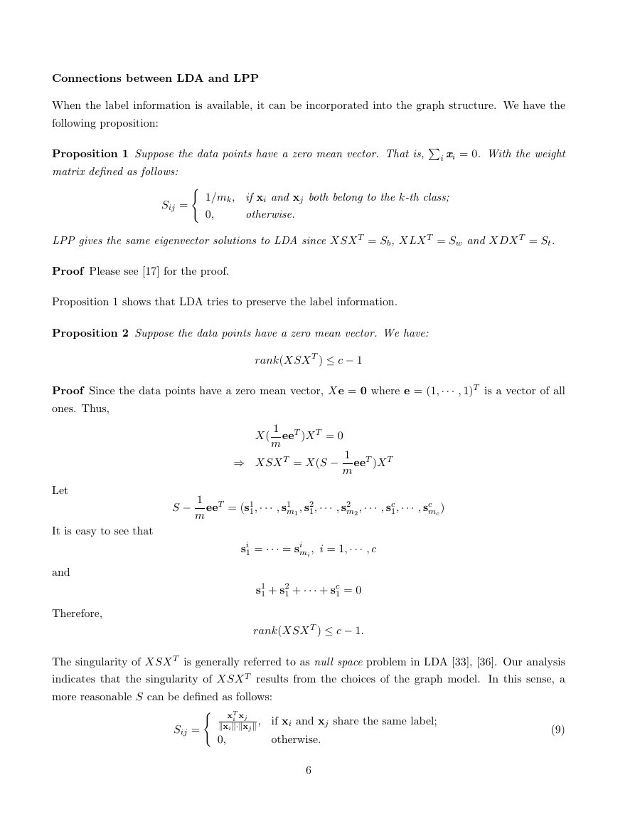
Proposition 2 Suppose the data points have a zero mean vector. We have:
rank(XSX T ) ≤ c − 1
Proof Since the data points have a zero mean vector, Xe = 0 where e = (1,··· , 1)T is a vector of all
ones. Thus,
X(
1
meeT )X T = 0
⇒ XSX T = X(S − 1
meeT )X T
Let
It is easy to see that
and
Therefore,
S − 1
meeT = (s1
1,··· , s1
m1
1,··· , s2
, s2
m2
,··· , sc
1,··· , sc
mc)
1 = ··· = si
si
mi
, i = 1,··· , c
s1
1 + s2
1 + ··· + sc
1 = 0
rank(XSX T ) ≤ c − 1.
The singularity of XSX T is generally referred to as null space problem in LDA [33], [36]. Our analysis
indicates that the singularity of XSX T results from the choices of the graph model. In this sense, a
more reasonable S can be defined as follows:
Sij =
xT
i xj
xi·xj ,
0,
if xi and xj share the same label;
otherwise.
(9)
6
�
or
Sij =
⎧⎨⎩ e− xi−xj2
t
0,
,
if xi and xj share the same label;
otherwise.
(10)
Clear, the above choices of S no longer suffer from the null space problem.
Connections Between LPP and PCA
Let x and y be two independent random variables in the data space. We first define a � Covariance
matrix C� as follows.
(x − y) (x − y)T |x − y < �
(x − E[x]) (x − E[x])T
Definition � Covariance Matrix:
C� =
1
2
Let us recall the standard covariance matrix:
Definition Covariance Matrix: C = E
We have the following propositions:
Proposition 3 lim�→∞ C� = C
E
Proposition 4 With the weight matrix defined as follows:
Sij =
if xi − xj < �
1,
0, otherwise.
(11)
We have: limm→∞ 1
m2β
XLX T = C�, where β = P rob(x − y < �).
Please see [15] for the proofs of the above propositions. These propositions indicate that the matrix
XLX T provides a statistical estimation of the � covariance matrix. Especially, when � tends to infinity,
XLX T is just the sample covariance matrix.
Our analysis indicates that the choices of different graph structure play the central role of LPP. In
some situations, one may incorporate prior information into the graph structure. For example, for web
graph, one may connect two pages if there is a hyperlink between them [26]. In general, one can apply
(9) for supervised learning and (11) for unsupervised learning.
3 Regularized LPP with Two-Dimensional Discretized Laplacian Smooth-
ing
In this section, we describe how to apply Laplacian penalized functional to measure the smoothness of
the basis vectors of the face space, which plays the key role in the regularized LPP with two-dimensional
discretized laplacian smoothing algorithm. We begin with a general description of Laplacian smoothing.
7
�




 2023年江西萍乡中考道德与法治真题及答案.doc
 2012年重庆南川中考生物真题及答案.doc
 2013年江西师范大学地理学综合及文艺理论基础考研真题.doc
 2020年四川甘孜小升初语文真题及答案I卷.doc
 2020年注册岩土工程师专业基础考试真题及答案.doc
 2023-2024学年福建省厦门市九年级上学期数学月考试题及答案.doc
 2021-2022学年辽宁省沈阳市大东区九年级上学期语文期末试题及答案.doc
 2022-2023学年北京东城区初三第一学期物理期末试卷及答案.doc
 2018上半年江西教师资格初中地理学科知识与教学能力真题及答案.doc
 2012年河北国家公务员申论考试真题及答案-省级.doc
 2020-2021学年江苏省扬州市江都区邵樊片九年级上学期数学第一次质量检测试题及答案.doc
 2022下半年黑龙江教师资格证中学综合素质真题及答案.doc