VBM Tutorial
John Ashburner
March 15, 2010
1 Getting Started
The data provided are a selection of T1-weighted scans from the freely available IXI dataset1.
Note that the scans were acquired in the saggital orientation, but a matrix in the NIfTI headers
encodes this information so SPM can treat them as axial.
The overall plan will be to
• Start up SPM.
• Check that the images are in a suitable format (Check Reg and Display buttons).
• Segment the images, to identify grey and white matter (using the SPM→Tools→New Seg-
ment option). Grey matter will eventually be warped to MNI space. This step also generates
“imported” images, which will be used in the next step.
• Estimate the deformations that best align the images together by iteratively registering the
imported images with their average (SPM→Tools→DARTEL Tools→Run DARTEL (create
Templates)).
• Generate spatially normalised and smoothed Jacobian scaled grey matter images, using the
deformations estimated in the previous step (SPM→Tools→DARTEL Tools→Normalise to
MNI Space).
• Do some statistics on the smoothed images (Basic models, Estimate and Results options).
The tutorial will use SPM8, which is is available from http://www.fil.ion.ucl.ac.uk/spm/.
This is the most recent version of the SPM software2. Normally, the software would be downloaded
and unpacked3, and the patches/fixes then downloaded and unpacked so that they overwrite the
original release. SPM8 should be installed, so there is no need to download it now.
SPM runs in the MATLAB package, which is worth learning how to program a little if you
ever plan to do any imaging research. Start MATLAB, and type “editpath”. This will give you a
window that allows you to tell MATLAB where to find the SPM8 software. More advanced users
could use the “path” command to do this.
You may then wish to change to the directory where the example data are stored.
SPM is started by typing “spm” or (eg) “spm pet”. This will pop open a bunch of windows.
The top-left one is the one with the buttons, but there are also a few options available via the
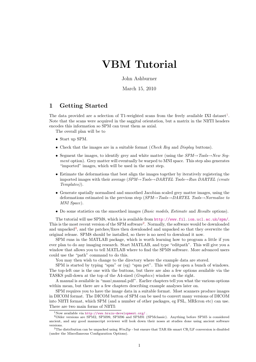
TASKS pull-down at the top of the A4-sized (Graphics) window on the right.
A manual is available in “man\manual.pdf”. Earlier chapters tell you what the various options
within mean, but there are a few chapters describing example analyses later on.
SPM requires you to have the image data in a suitable format. Most scanners produce images
in DICOM format. The DICOM button of SPM can be used to convert many versions of DICOM
into NIfTI format, which SPM (and a number of other packages, eg FSL, MRIcron etc) can use.
There are two main forms of NIfTI:
1Now available via http://www.brain-development.org/ .
2Older versions are SPM2, SPM99, SPM96 and SPM91 (SPMclassic). Anything before SPM5 is considered
ancient, and any good manuscript reviewer will look down their noses at studies done using ancient software
versions.
3The distribution can be unpacked using WinZip - but ensure that TAR file smart CR/LF conversion is disabled
(under the Miscellaneous Configuration Options).
1
�
1 GETTING STARTED
2
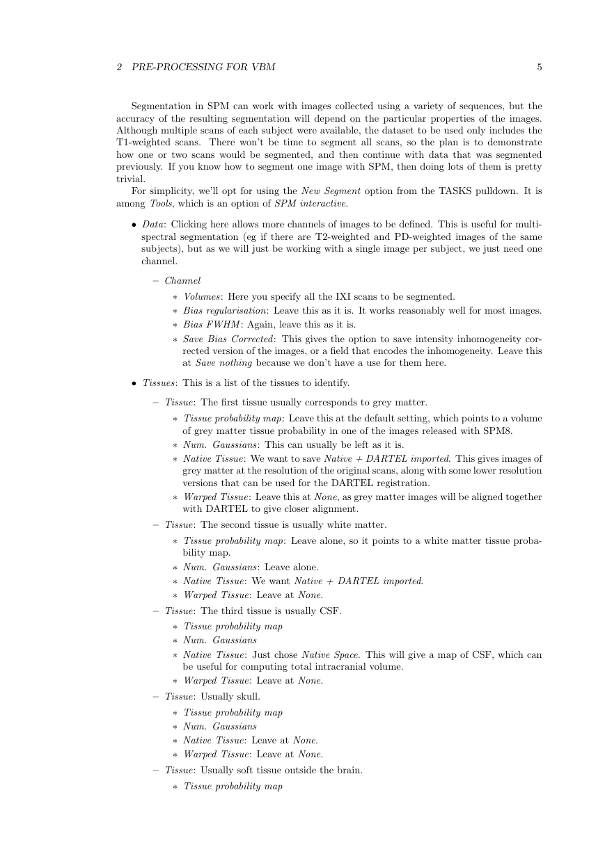
Figure 1: The TASKS pulldown.
• “.hdr” and “.img” files, which appear superficially similar to the older ANALYZE format.
The .img file contains the actual image data, and the .hdr contains the information necessary
for programs to understand it.
• “.nii” files, which combines all the information into one file.
NIfTI files have some orientation information in them, but sometimes this needs “improving”.
Ensure that the images are approximately aligned with MNI space. This makes it easier to align
the data with MNI space, using local optimisation procedures such as those in SPM. NIfTI images
can be single 3D volumes, but 4D or even 5D images are possible. For SPM5 onwards, the 4D
images may have an additional “.mat” file. 3D volumes generated by older SPM versions may
also have a “.mat” file associated with them.
1.1 Check Reg button
Click the button and select one (or more) of the original IXI scans, as well as the “canonical\avg152T1.nii”
file in the SPM release. This shows the relative positions of the images, as understood by SPM.
Note that if you click the right mouse button on one of the images, you will be shown a menu of
options, which you may wish to try. If images need to be rotated or translated (shifted), then this
can be done using the Display button. Before you begin, each image should be approximately
aligned within about 5cm and about 20 degrees of the template data released with SPM.
1.2 Display button
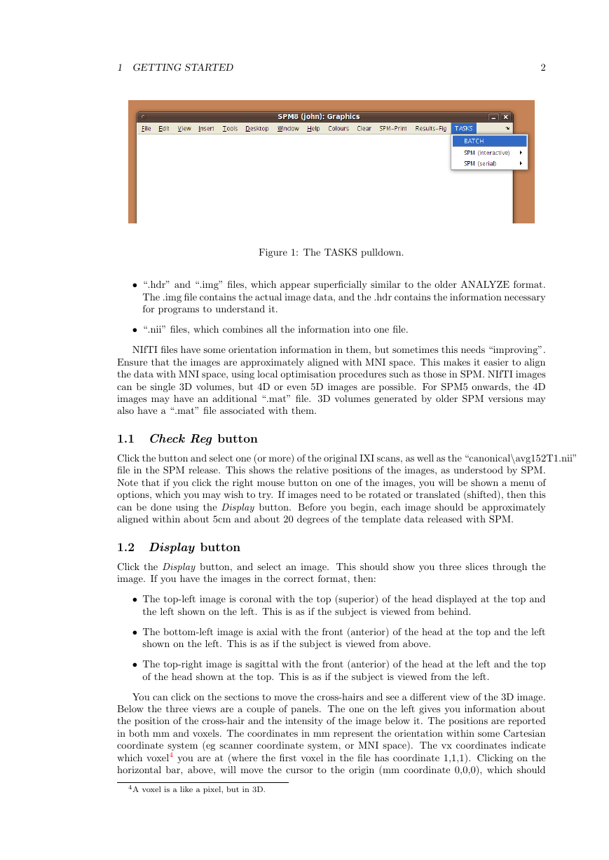
Click the Display button, and select an image. This should show you three slices through the
image. If you have the images in the correct format, then:
• The top-left image is coronal with the top (superior) of the head displayed at the top and
the left shown on the left. This is as if the subject is viewed from behind.
• The bottom-left image is axial with the front (anterior) of the head at the top and the left
shown on the left. This is as if the subject is viewed from above.
• The top-right image is sagittal with the front (anterior) of the head at the left and the top
of the head shown at the top. This is as if the subject is viewed from the left.
You can click on the sections to move the cross-hairs and see a different view of the 3D image.
Below the three views are a couple of panels. The one on the left gives you information about
the position of the cross-hair and the intensity of the image below it. The positions are reported
in both mm and voxels. The coordinates in mm represent the orientation within some Cartesian
coordinate system (eg scanner coordinate system, or MNI space). The vx coordinates indicate
which voxel4 you are at (where the first voxel in the file has coordinate 1,1,1). Clicking on the
horizontal bar, above, will move the cursor to the origin (mm coordinate 0,0,0), which should
4A voxel is a like a pixel, but in 3D.
�
1 GETTING STARTED
3
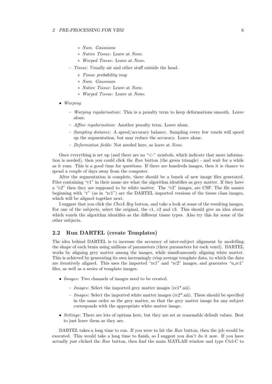
Figure 2: Check Reg and Display.
be close(ish) to the anterior cingulate (AC). The intensity at the point in the image below the
cross-hairs is obtained by interpolation of the neighbouring voxels. This means that for a binary
image, the intensity may not be shown as exactly 0 or 1.
Below this are a number of boxes that allow the image to be re-oriented and shifted. If you
click on the AC, you can see its mm coordinates. The objective is to move this point to a position
close to 0,0,0. To do this, you would translate the images by minus the mm coordinates shown
for the AC. These values would be entered into the right {mm}, forward {mm} and up {mm}
boxes.
If rotations are needed, they can be entered into rotation boxes. Notice that the angles are
specified in radians, so a rotation of 90 degrees would be entered as “1.5708” or as “pi/2”. When
entering rotations around different axes, the result can be a bit confusing, so some trial and error
may be needed. Note that “pitch” refers to rotations about the x axis, “roll” is for rotations
about the y axis and “yaw” is for rotations about the z axis5.
To actually change the header of the image, you can use the Reorient images... button. This
allows you to select multiple images, and they would all be rotated and translated in the same
way.
Very occasionally, you may need to flip the images. This can be achieved by entering a “-1”
in one of the “resize” boxes.
The panel on the right shows various pieces of information about the image being displayed.
Note that images can be represented by various datatypes. Integer datatypes can only encode a
limited range of values, and are usually used to save some disk space. For example, the “uint8”
datatype can only encode integer values from 0 to 255, and the “int16” datatype can only encode
values from -32768 to 32767. For this reason, there is also a scale-factor (and sometimes a constant
term) saved in the headers in order to make the values more quantitative. For example, a uint8
datatype may be used to save an image of probabilities, which can take values from 0.0 to 1.0.
5In aeronautics, pitch, roll and yaw would be defined differently, but that is because they use a different labelling
of their axes.
�
2 PRE-PROCESSING FOR VBM
4
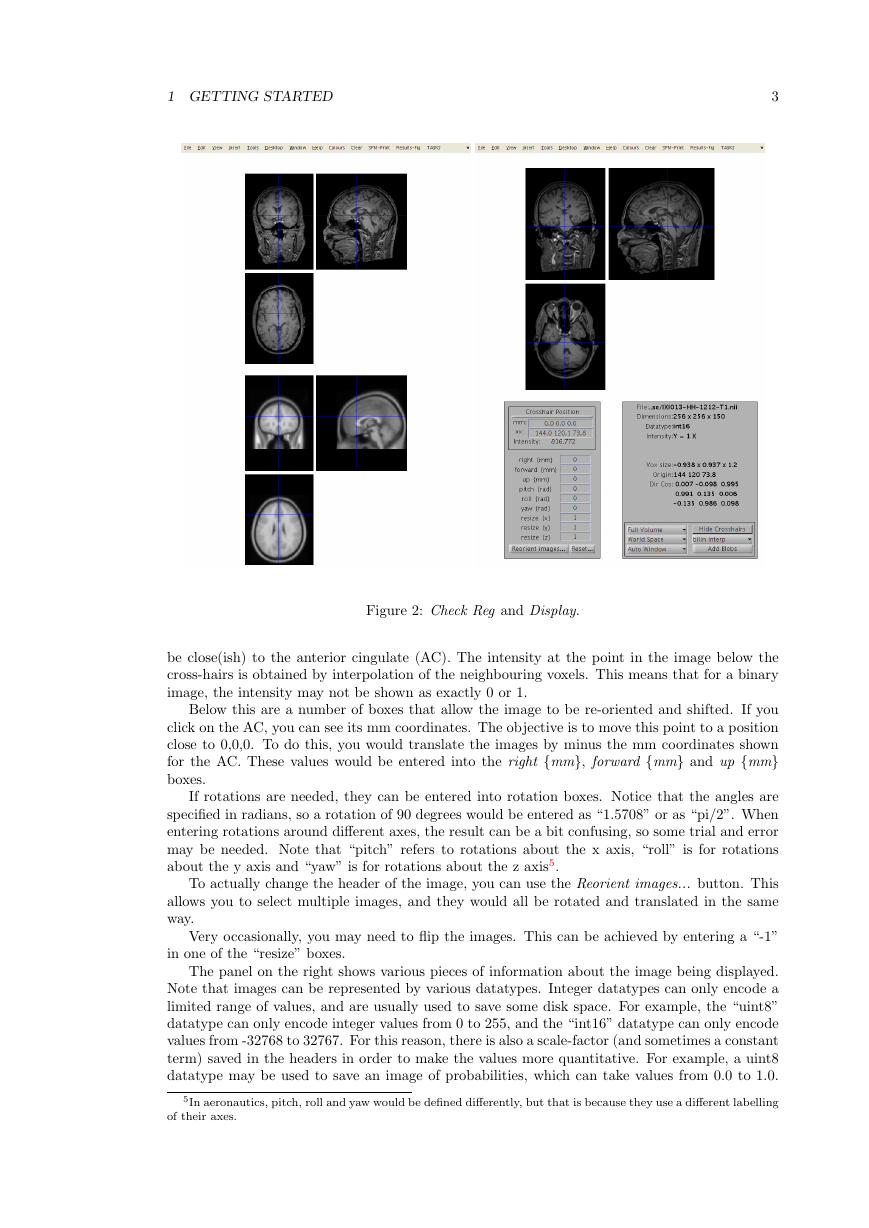
Figure 3: Left- and right-handed coordinate systems.
This would use a scale-factor of 1/255.
Below this lot is some positional and voxel size information. Note that the first element of the
voxel sizes may be negative. This indicates whether there is a reflection between the coordinate
system of the voxels and the mm coordinate system. One of them is right-handed, whereas the
other is left-handed.
Another option allows the image to be zoomed to a region around the cross-hair. The effects of
changing the interpolation are most apparent when the image is zoomed up. Also, if the original
image was collected in a different orientation, then the image can be viewed in Native Space (as
opposed to World Space), to show it this way.
2 Pre-processing for VBM
At this point, the images should all be in a suitable format for SPM to work with them. The
following procedures will be used. For the tutorial, you should specify them one at a time. In
practice though, it is much easier to use the batching system of SPM. The sequence of jobs (use
the TASKS pull-down from the Graphics window to select BATCH ) would be:
• Module List
– SPM→Tools→New Segment: To generate the roughly (via a rigid-body) aligned
grey and white matter images of the subjects.
– SPM→Tools→DARTEL Tools→Run DARTEL (create Template): Determine
the nonlinear deformations for warping all the grey and white matter images so that
they match each other.
– SPM→Tools→DARTEL Tools→Normalise to MNI Space: Actually generate
the smoothed “modulated” warped grey and white matter images.
2.1 Using Tools→New Segment
The objective now is to automatically identify different tissue types within the images, using the
New Segment option. The output of the segmentation will be used for achieving more accurate
inter-subject alignment using DARTEL (to be explained later). This new segmentation option in
SPM8 can be found within SPM→Tools→New Segment. It is also suggested that Native Space
versions of the tissues in which you are interested are generated, along with “DARTEL imported”
versions of grey and white matter. For VBM, the native space images are usually the c1*.nii files,
as it is these images that will eventually be warped to MNI space. Both the imported and native
tissue class image sets can be specified via the Native Space options of the user interface.
�
2 PRE-PROCESSING FOR VBM
5
Segmentation in SPM can work with images collected using a variety of sequences, but the
accuracy of the resulting segmentation will depend on the particular properties of the images.
Although multiple scans of each subject were available, the dataset to be used only includes the
T1-weighted scans. There won’t be time to segment all scans, so the plan is to demonstrate
how one or two scans would be segmented, and then continue with data that was segmented
previously. If you know how to segment one image with SPM, then doing lots of them is pretty
trivial.
For simplicity, we’ll opt for using the New Segment option from the TASKS pulldown. It is
among Tools, which is an option of SPM interactive.
• Data: Clicking here allows more channels of images to be defined. This is useful for multi-
spectral segmentation (eg if there are T2-weighted and PD-weighted images of the same
subjects), but as we will just be working with a single image per subject, we just need one
channel.
– Channel
∗ Volumes: Here you specify all the IXI scans to be segmented.
∗ Bias regularisation: Leave this as it is. It works reasonably well for most images.
∗ Bias FWHM : Again, leave this as it is.
∗ Save Bias Corrected: This gives the option to save intensity inhomogeneity cor-
rected version of the images, or a field that encodes the inhomogeneity. Leave this
at Save nothing because we don’t have a use for them here.
• Tissues: This is a list of the tissues to identify.
– Tissue: The first tissue usually corresponds to grey matter.
of grey matter tissue probability in one of the images released with SPM8.
∗ Tissue probability map: Leave this at the default setting, which points to a volume
∗ Num. Gaussians: This can usually be left as it is.
∗ Native Tissue: We want to save Native + DARTEL imported. This gives images of
grey matter at the resolution of the original scans, along with some lower resolution
versions that can be used for the DARTEL registration.
∗ Warped Tissue: Leave this at None, as grey matter images will be aligned together
with DARTEL to give closer alignment.
– Tissue: The second tissue is usually white matter.
bility map.
∗ Tissue probability map: Leave alone, so it points to a white matter tissue proba-
∗ Num. Gaussians: Leave alone.
∗ Native Tissue: We want Native + DARTEL imported.
∗ Warped Tissue: Leave at None.
– Tissue: The third tissue is usually CSF.
∗ Tissue probability map
∗ Num. Gaussians
∗ Native Tissue: Just chose Native Space. This will give a map of CSF, which can
∗ Warped Tissue: Leave at None.
be useful for computing total intracranial volume.
– Tissue: Usually skull.
∗ Tissue probability map
∗ Num. Gaussians
∗ Native Tissue: Leave at None.
∗ Warped Tissue: Leave at None.
– Tissue: Usually soft tissue outside the brain.
∗ Tissue probability map
�
2 PRE-PROCESSING FOR VBM
6
∗ Num. Gaussians
∗ Native Tissue: Leave at None.
∗ Warped Tissue: Leave at None.
– Tissue: Usually air and other stuff outside the head.
∗ Tissue probability map
∗ Num. Gaussians
∗ Native Tissue: Leave at None.
∗ Warped Tissue: Leave at None.
• Warping
– Warping regularisation: This is a penalty term to keep deformations smooth. Leave
alone.
– Affine regularisation: Another penalty term. Leave alone.
– Sampling distance: A speed/accuracy balance. Sampling every few voxels will speed
up the segmentation, but may reduce the accuracy. Leave alone.
– Deformation fields: Not needed here, so leave at None.
Once everything is set up (and there are no “<-” symbols, which indicate that more informa-
tion is needed), then you could click the Run button (the green triangle) - and wait for a while
as it runs. This is a good time for questions. If there are hundreds images, then it is chance to
spend a couple of days away from the computer.
After the segmentation is complete, there should be a bunch of new image files generated.
Files containing “c1” in their name are what the algorithm identifies as grey matter. If they have
a “c2” then they are supposed to be white matter. The “c3” images, are CSF. The file names
beginning with “r” (as in “rc1”) are the DARTEL imported versions of the tissue class images,
which will be aligned together next.
I suggest that you click the Check Reg button, and take a look at some of the resulting images.
For one of the subjects, select the original, the c1, c2 and c3. This should give an idea about
which voxels the algorithm identifies as the different tissue types. Also try this for some of the
other subjects.
2.2 Run DARTEL (create Templates)
The idea behind DARTEL is to increase the accuracy of inter-subject alignment by modelling
the shape of each brain using millions of parameters (three parameters for each voxel). DARTEL
works by aligning grey matter among the images, while simultaneously aligning white matter.
This is achieved by generating its own increasingly crisp average template data, to which the data
are iteratively aligned. This uses the imported “rc1” and “rc2” images, and generates “u rc1”
files, as well as a series of template images.
• Images: Two channels of images need to be created.
– Images: Select the imported grey matter images (rc1*.nii).
– Images: Select the imported white matter images (rc2*.nii). These should be specified
in the same order as the grey matter, so that the grey matter image for any subject
corresponds with the appropriate white matter image.
• Settings: There are lots of options here, but they are set at reasonable default values. Best
to just leave them as they are.
DARTEL takes a long time to run. If you were to hit the Run button, then the job would be
executed. This would take a long time to finish, so I suggest you don’t do it now. If you have
actually just clicked the Run button, then find the main MATLAB window and type Ctrl-C to
�
2 PRE-PROCESSING FOR VBM
7
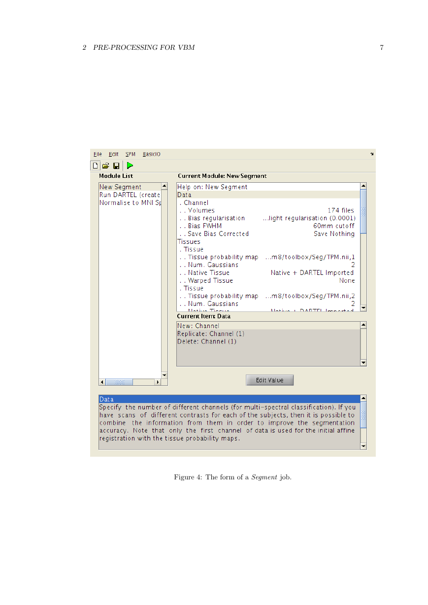
Figure 4: The form of a Segment job.
�
2 PRE-PROCESSING FOR VBM
8
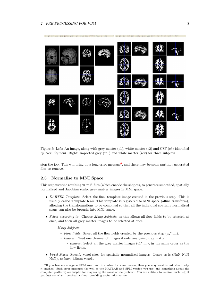
Figure 5: Left: An image, along with grey matter (c1), white matter (c2) and CSF (c3) identified
by New Segment. Right: Imported grey (rc1) and white matter (rc2) for three subjects.
stop the job. This will bring up a long error message6, and there may be some partially generated
files to remove.
2.3 Normalise to MNI Space
This step uses the resulting ‘u rc1” files (which encode the shapes), to generate smoothed, spatially
normalised and Jacobian scaled grey matter images in MNI space.
• DARTEL Template: Select the final template image created in the previous step. This is
usually called Template 6.nii. This template is registered to MNI space (affine transform),
allowing the transformations to be combined so that all the individual spatially normalised
scans can also be brought into MNI space.
• Select according to: Choose Many Subjects, as this allows all flow fields to be selected at
once, and then all grey matter images to be selected at once.
– Many Subjects
∗ Flow fields: Select all the flow fields created by the previous step (u *.nii).
∗ Images: Need one channel of images if only analysing grey matter.
· Images: Select all the grey matter images (c1*.nii), in the same order as the
flow fields.
• Voxel Sizes: Specify voxel sizes for spatially normalised images. Leave as is (NaN NaN
NaN), to have 1.5mm voxels.
6If you become a regular SPM user, and it crashes for some reason, then you may want to ask about why
it crashed. Such error messages (as well as the MATLAB and SPM version you use, and something about the
computer platform) are helpful for diagnosing the cause of the problem. You are unlikely to receive much help if
you just ask why it crashed, without providing useful information.
�


 2023年江西萍乡中考道德与法治真题及答案.doc
 2012年重庆南川中考生物真题及答案.doc
 2013年江西师范大学地理学综合及文艺理论基础考研真题.doc
 2020年四川甘孜小升初语文真题及答案I卷.doc
 2020年注册岩土工程师专业基础考试真题及答案.doc
 2023-2024学年福建省厦门市九年级上学期数学月考试题及答案.doc
 2021-2022学年辽宁省沈阳市大东区九年级上学期语文期末试题及答案.doc
 2022-2023学年北京东城区初三第一学期物理期末试卷及答案.doc
 2018上半年江西教师资格初中地理学科知识与教学能力真题及答案.doc
 2012年河北国家公务员申论考试真题及答案-省级.doc
 2020-2021学年江苏省扬州市江都区邵樊片九年级上学期数学第一次质量检测试题及答案.doc
 2022下半年黑龙江教师资格证中学综合素质真题及答案.doc