System Identification
System Identification
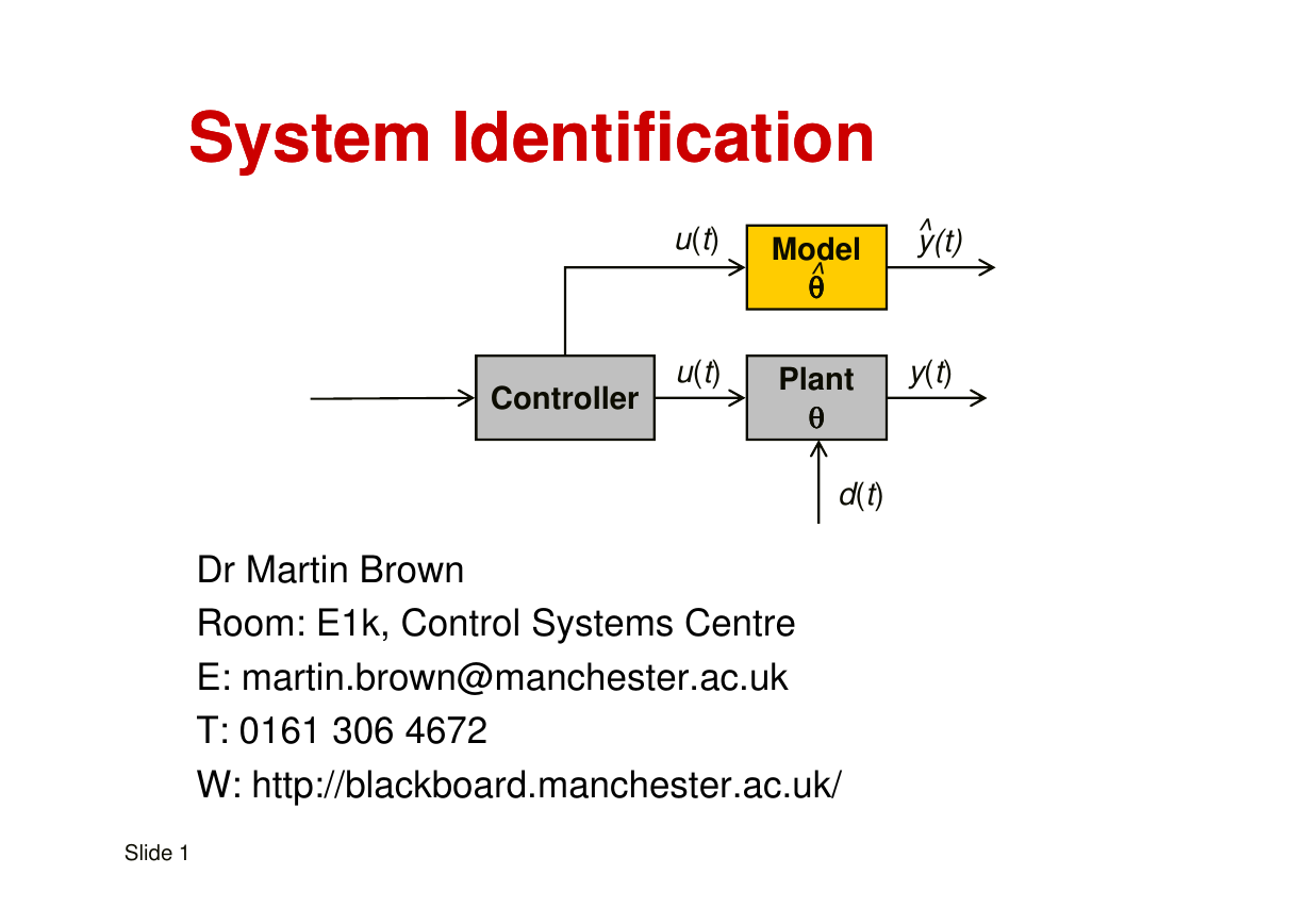
u(t)
u(t)
y(t)^
y(t)
Model
^
θθθθ
Plant
θθθθ
d(t)
Controller
Dr Martin Brown
Room: E1k, Control Systems Centre
E: martin.brown@manchester.ac.uk
T: 0161 306 4672
W: http://blackboard.manchester.ac.uk/
Slide 1
�
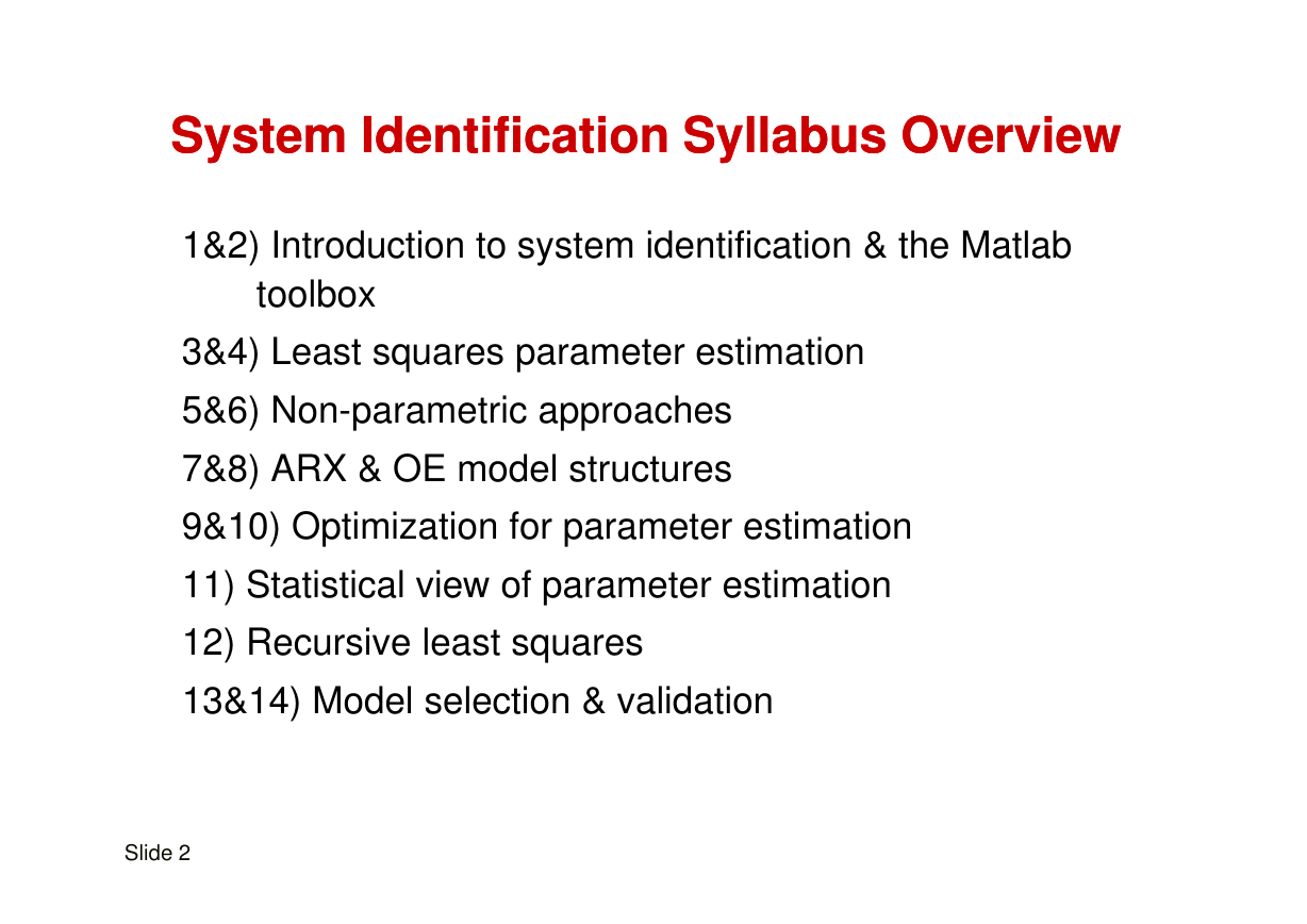
System Identification Syllabus Overview
System Identification Syllabus Overview
1&2) Introduction to system identification & the Matlab
toolbox
3&4) Least squares parameter estimation
5&6) Non-parametric approaches
7&8) ARX & OE model structures
7&8) ARX & OE model structures
9&10) Optimization for parameter estimation
11) Statistical view of parameter estimation
12) Recursive least squares
13&14) Model selection & validation
Slide 2
�
Lectures 1&2) An Introduction to System
Lectures 1&2)
An Introduction to System
Identification
Identification
a) Review of dynamic systems, including discrete time.
b)
Introduction to system identification
c) System identification exemplar problems
� RC circuit (electrical – CT & DT)
�
�
Solar heating
Solar heating
d)
Introduction to Matlab data generation and the System
Identification toolbox
1
0.5
)uk
t
(
x
yk
)
t
(
y
0
-10
1.4
1.2
1
0.8
0.6
0.4
0.2
0
-10
0
10
20
30
40
50
60
t
0
10
20
30
40
50
60
t
Slide 3
ˆ
y
k
−
0.94
y
k
−
1
=
0.27
u
k
−
1
�
1a) System & Model Definition
1a) System & Model Definition
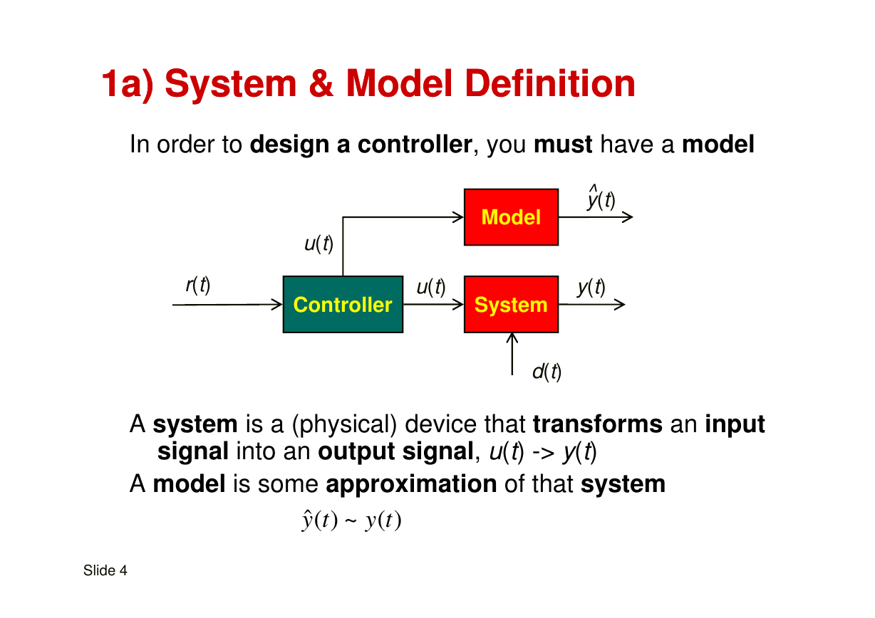
In order to design a controller, you must have a model
y(t)^
Model
u(t)
r(t)
Controller
Controller
u(t)
y(t)
System
System
d(t)
A system is a (physical) device that transforms an input
signal into an output signal, u(t) -> y(t)
A model is some approximation of that system
ˆ( ) ~ ( )
y t
y t
Slide 4
�
1a) How are Models Used?
1a) How are Models Used?
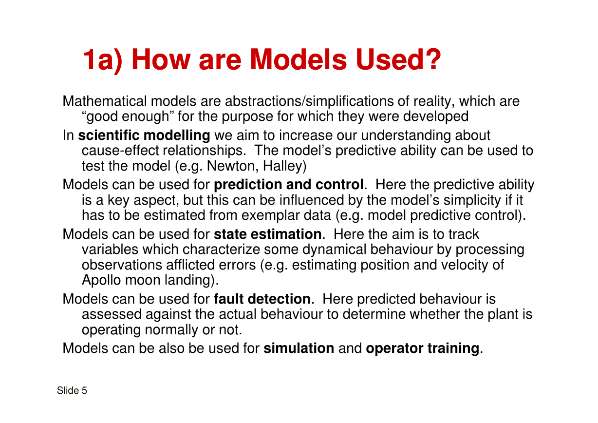
Mathematical models are abstractions/simplifications of reality, which are
“good enough” for the purpose for which they were developed
In scientific modelling we aim to increase our understanding about
cause-effect relationships. The model’s predictive ability can be used to
test the model (e.g. Newton, Halley)
Models can be used for prediction and control. Here the predictive ability
is a key aspect, but this can be influenced by the model’s simplicity if it
has to be estimated from exemplar data (e.g. model predictive control).
has to be estimated from exemplar data (e.g. model predictive control).
Models can be used for state estimation. Here the aim is to track
variables which characterize some dynamical behaviour by processing
observations afflicted errors (e.g. estimating position and velocity of
Apollo moon landing).
Models can be used for fault detection. Here predicted behaviour is
assessed against the actual behaviour to determine whether the plant is
operating normally or not.
Models can be also be used for simulation and operator training.
Slide 5
�
1a) Example Models/Systems
1a) Example Models/Systems
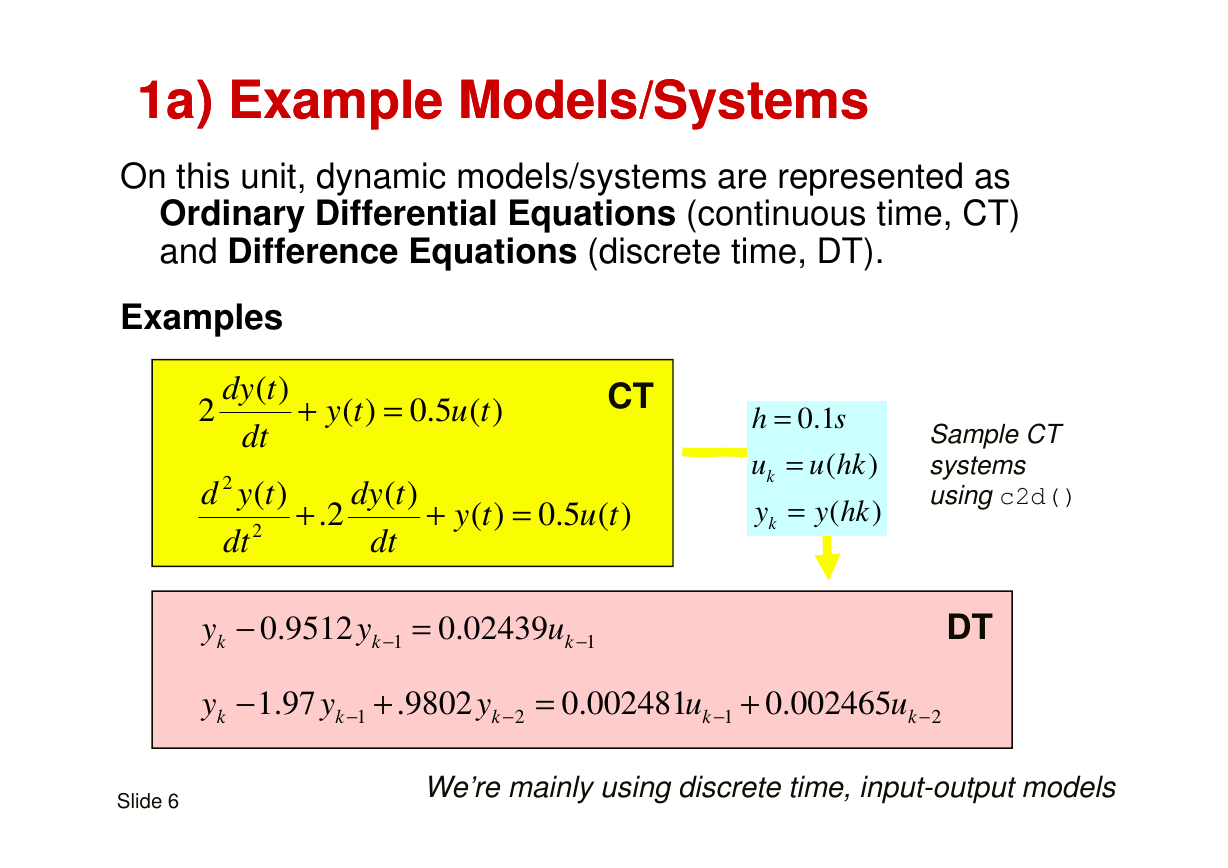
On this unit, dynamic models/systems are represented as
Ordinary Differential Equations (continuous time, CT)
and Difference Equations (discrete time, DT).
Examples
2
( )
dy t
dt
dt
+
y t
( ) 0.5 ( )
u t
=
CT
2
( )
d y t
2
dt
+
.2
( )
dy t
dt
+
y t
( ) 0.5 ( )
u t
=
h
h
=
=
0.1
0.1
s
s
u
k
y
k
=
u hk
(
)
=
y hk
(
)
Sample CT
Sample CT
systems
using c2d()
y
k
y
k
−
0.9512
y
k
−
1
=
0.02439
u
k
−
1
DT
−
1.97
y
k
−
1
+
.9802
y
k
−
2
=
0.002481
u
k
−
1
+
0.002465
u
k
−
2
Slide 6
We’re mainly using discrete time, input-output models
�
1a) Using Models Example:
1a) Using Models Example:
PI Controller Design
PI Controller Design
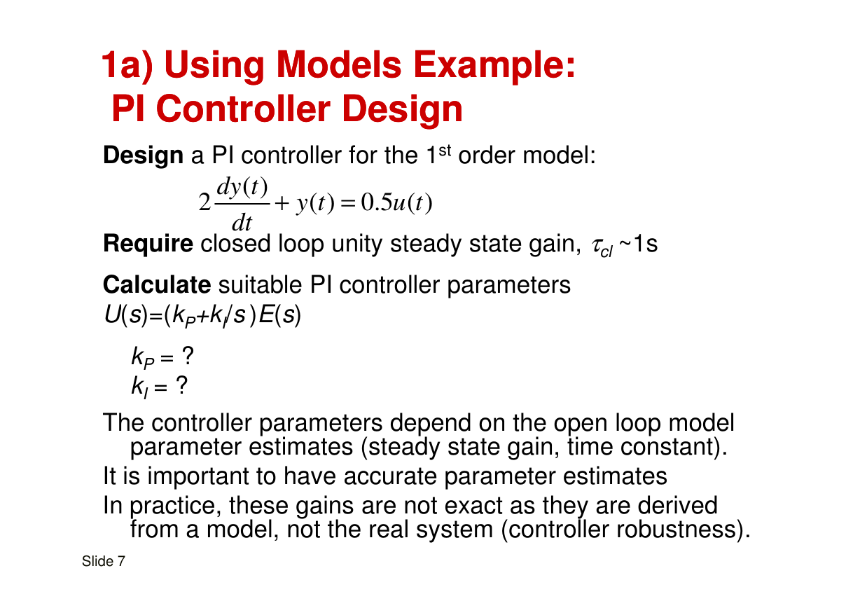
Design a PI controller for the 1st order model:
( )
dy t
2
+
y t
( ) 0.5 ( )
u t
=
dt
Require closed loop unity steady state gain, τcl ~1s
Calculate suitable PI controller parameters
U(s)=(k +k /s )E(s)
U(s)=(kP+kI/s )E(s)
kP = ?
kI = ?
The controller parameters depend on the open loop model
parameter estimates (steady state gain, time constant).
It is important to have accurate parameter estimates
In practice, these gains are not exact as they are derived
from a model, not the real system (controller robustness).
Slide 7
�
1a) What is a Dynamic System?
1a) What is a Dynamic System?
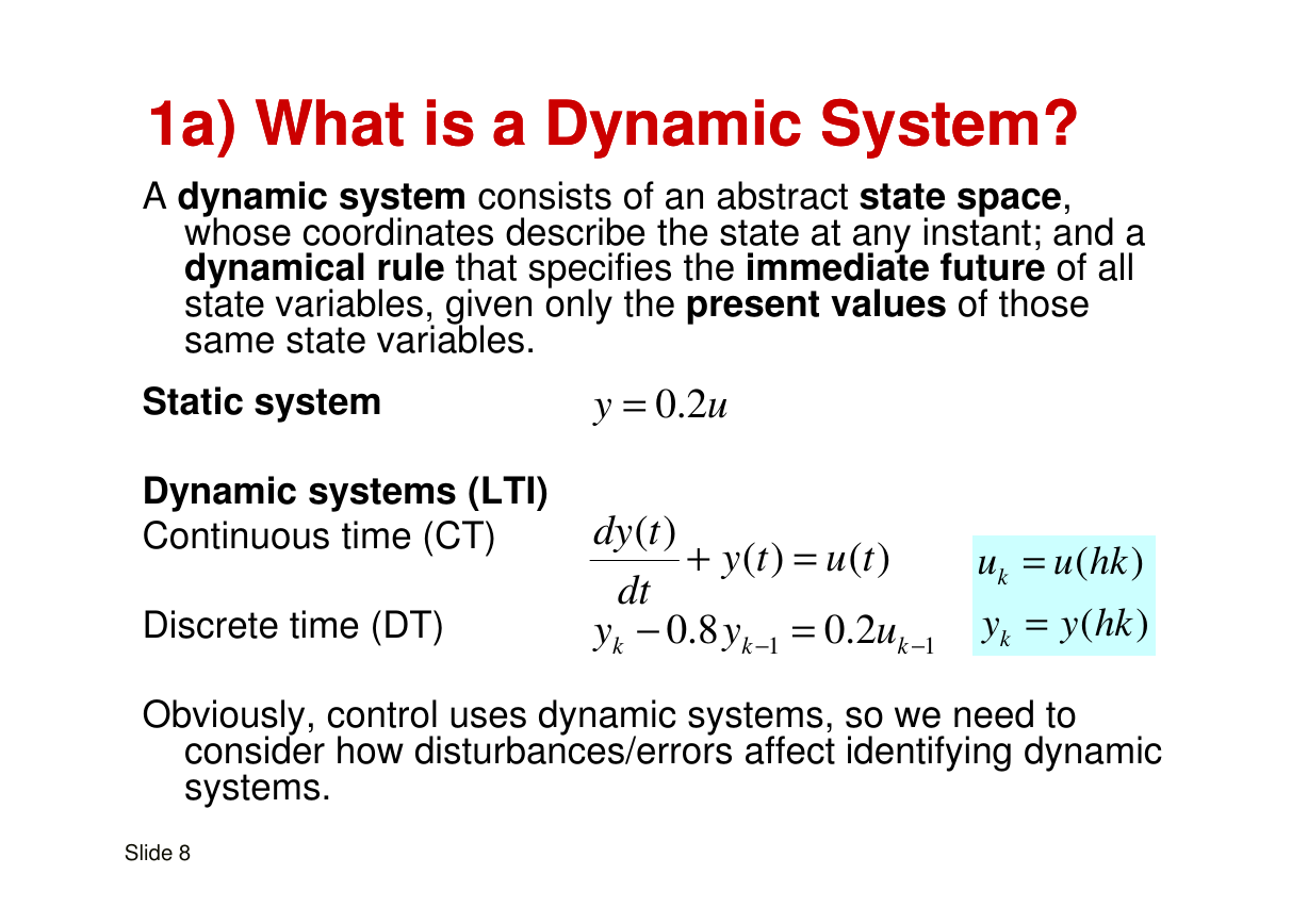
A dynamic system consists of an abstract state space,
whose coordinates describe the state at any instant; and a
dynamical rule that specifies the immediate future of all
state variables, given only the present values of those
same state variables.
Static system
y
=
0.2
u
Dynamic systems (LTI)
Continuous time (CT)
( )
dy t
Discrete time (DT)
dt
−
k
y
0.8
y
k
−
1
=
0.2
u
k
−
1
+
( )
y t
=
( )
u t
u
k
y
k
=
u hk
(
)
=
y hk
(
)
Obviously, control uses dynamic systems, so we need to
consider how disturbances/errors affect identifying dynamic
systems.
Slide 8
�



 2023年江西萍乡中考道德与法治真题及答案.doc
 2012年重庆南川中考生物真题及答案.doc
 2013年江西师范大学地理学综合及文艺理论基础考研真题.doc
 2020年四川甘孜小升初语文真题及答案I卷.doc
 2020年注册岩土工程师专业基础考试真题及答案.doc
 2023-2024学年福建省厦门市九年级上学期数学月考试题及答案.doc
 2021-2022学年辽宁省沈阳市大东区九年级上学期语文期末试题及答案.doc
 2022-2023学年北京东城区初三第一学期物理期末试卷及答案.doc
 2018上半年江西教师资格初中地理学科知识与教学能力真题及答案.doc
 2012年河北国家公务员申论考试真题及答案-省级.doc
 2020-2021学年江苏省扬州市江都区邵樊片九年级上学期数学第一次质量检测试题及答案.doc
 2022下半年黑龙江教师资格证中学综合素质真题及答案.doc