�
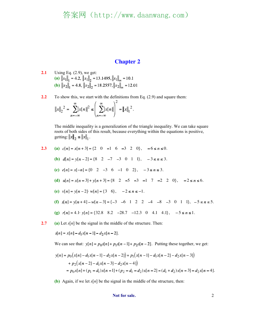
2.1 Using Eq. (2.9), we get:
(a)
=
=
(b)
Chapter 2
=
2.2
To show this, we start with the definitions from Eq. (2.9) and square them:
2
2
2
[ ]
[ ]
2
2 .
1
The middle inequality is a generalization of the triangle inequality. We can take square
roots of both sides of this result, because everything within the equations is positive,
getting:
2.3
2.7
(a) [ ] = [ + 3] = {2 0
1 6
3 2 0},
(b)
[ ] = [
2] = {8 2
7
3 0 11},
6
3
0.
3.
(c) [ ] = [
] = {0 2
3 6
1 0 2},
3
3.
(d) [ ] = [
3] + [ + 3] = {8 2
5
3
1 7
2 2 0},
2
6.
(e) [ ] = [
2]
[ ] = {3 6}, 2
1.
(f) [ ] = [ + 4]
[
3] = { 3
612 2
4
8
3 0 11},
5
5.
(g) [ ] = 4.1 [ ] = {32.8 8.2
28.7
12.3 0 4.1 4.1}, 5
1.
(a) Let [] be the signal in the middle of the structure. Then:
We can see that:
=
+
+
. Putting these together, we get:
[ ] = 0
(
[ ]
1 [
1]
2 [
2]
) + 1
(
[
1]
1 [
2]
2 [
)
3]
(
[
2]
1 [
3]
+ 2
= 0 [ ] + ( 1
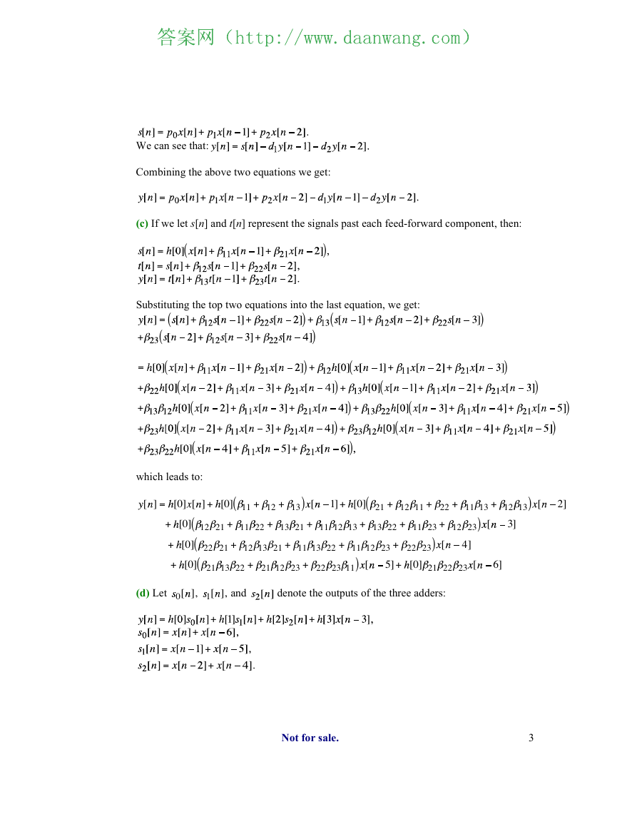
(b) Again, if we let [] be the signal in the middle of the structure, then:
2 [
1] + ( 2
( 1 + 2) [
2) [
1) [
2]
1
)
4]
3]
2 [
4].
Not for sale.
2
+
+
=
Combining the above two equations we get:
=
+
+
(c) If we let [] and [] represent the signals past each feed-forward component, then:
(
+
+
+
+
+
+
)
=
We can see that:
=
=
=
(
=
(
Substituting the top two equations into the last equation, we get:
+
+
+
(
(
+
+
+
) +
)
) +
+
+
+
+
+
+
+
+
(
+
+
)
+
(
+
(
+
+
+
)
+
)
(
+
+
)
)
) +
) +
(
) +
)
(
(
(
+
=
+
+
+
+
which leads to:
[ ] = [0] [ ] + [0] 11 + 12 + 13
(
) [
(
1] + [0]
21 + 12 11 + 22 + 11 13 + 12 13
) [
2]
+ [0] 12 21 + 11 22 + 13 21 + 11 12 13 + 13 22 + 11 23 + 12 23
) [
3]
(
(
+ [0]
(
+ [0]
22 21 + 12 13 21 + 11 13 22 + 11 12 23 + 22 23
) [
4]
21 13 22 + 21 12 23 + 22 23 11
) [
5] + [0] 21 22 23 [
6]
(d) Let 0[ ], 1[ ], and
denote the outputs of the three adders:
=
=
=
=
+
+
+
+
+
+
Not for sale.
3
�
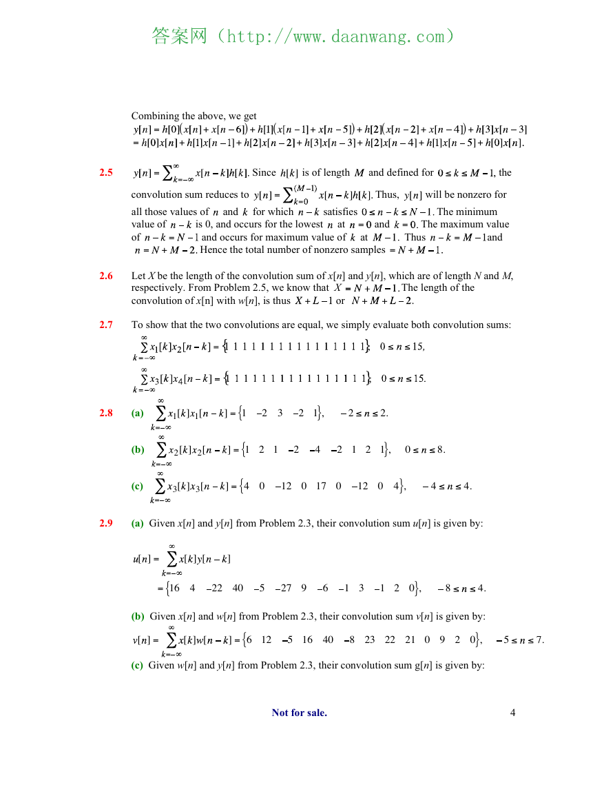
Combining the above, we get
=
=
=
(
+
=
+
) +
(
+
+
+
(
) +
+
+
+
) +
+
Since
is of length
and defined for
the
convolution sum reduces to
=
=
Thus,
will be nonzero for
and
for which
satisfies
The minimum
all those values of
value of
of
=
=
+
is 0, and occurs for the lowest
at = and = The maximum value
and occurs for maximum value of
Hence the total number of nonzero samples =
at
Thus
+
=
and
Let be the length of the convolution sum of [] and [], which are of length and ,
respectively. From Problem 2.5, we know that
convolution of [n] with [], is thus
The length of the
or +
+
+
To show that the two convolutions are equal, we simply evaluate both convolution sums:
2.5
2.6
2.7
2.8
(a)
1[ ] 1[
]
{
= 1
2 3
2 1
},
2
2.
=
=
=
(b)
(c)
2[ ] 2[
]
= 1 2 1
{
2
4
212 1
}, 0
8.
3[ ] 3[
]
= 4 0
{
12017 0
120 4
},
4
4.
(a) Given [] and [] from Problem 2.3, their convolution sum [] is given by:
[ ] =
[ ] [
]
=
{
= 16 4
2240
5
27 9
6
1 3
12 0
},
8
4.
(b) Given [] and [] from Problem 2.3, their convolution sum [] is given by:
[ ] =
[ ]
[
]
{
= 6 12
51640
82322210 92 0
},
5
7.
=
(c) Given [] and [] from Problem 2.3, their convolution sum g[ ] is given by:
2.9
Not for sale.
4
�
[ ] =
[ ] [
]
=
{
= 2454
17
374152
19
53
245127 1
},
7
5.
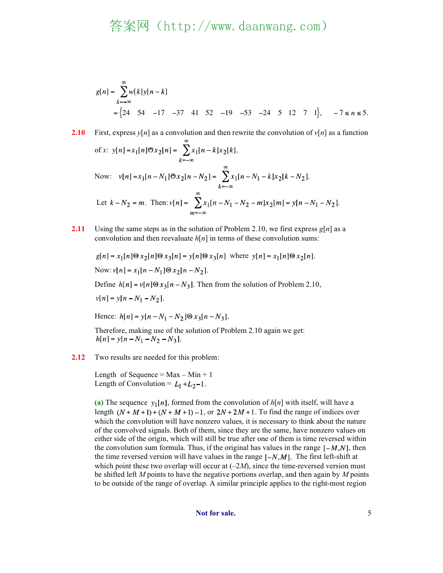
2.10 First, express [] as a convolution and then rewrite the convolution of [] as a function
of :
=
Now:
=
=
=
=
=
Let
=
Then:
=
=
=
2.11 Using the same steps as in the solution of Problem 2.10, we first express [] as a
convolution and then reevaluate [] in terms of these convolution sums:
=
=
where
=
Now:
=
Define
=
=
Then from the solution of Problem 2.10,
Hence:
=
Therefore, making use of the solution of Problem 2.10 again we get:
=
2.12
+
+
+
+ +
+
+
, formed from the convolution of [] with itself, will have a
Two results are needed for this problem:
Length of Sequence = Max — Min + 1
Length of Convolution =
(a) The sequence
length
which the convolution will have nonzero values, it is necessary to think about the nature
of the convolved signals. Both of them, since they are the same, have nonzero values on
either side of the origin, which will still be true after one of them is time reversed within
the convolution sum formula. Thus, if the original has values in the range
, then
the time reversed version will have values in the range
which point these two overlap will occur at (—2 ), since the time-reversed version must
be shifted left points to have the negative portions overlap, and then again by points
to be outside of the range of overlap. A similar principle applies to the right-most region
+ . To find the range of indices over
The first left-shift at
, or
Not for sale.
5
�
of overlap. The time-reversed signal must be shifted by twice to the right to be just
outside of the region of overlap, so that the right-most boundary of the resulting
convolution is (2). Therefore the convolution is nonzero in the range [—2 , 2].
Note that these boundaries also give the correct length of the resulting signal:
(2) — (—2) + 1 = 2 + 2 + 1.
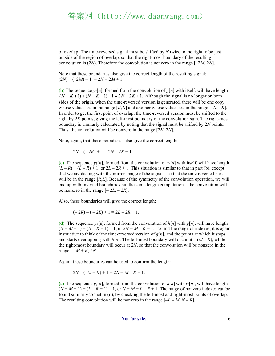
(b) The sequence 2[], formed from the convolution of [] with itself, will have length
Although the signal is no longer on both
sides of the origin, when the time-reversed version is generated, there will be one copy
whose values are in the range [ ,] and another whose values are in the range [— , —].
In order to get the first point of overlap, the time-reversed version must be shifted to the
right by 2 points, giving the left-most boundary of the convolution sum. The right-most
boundary is similarly calculated by noting that the signal must be shifted by 2 points.
Thus, the convolution will be nonzero in the range [2 , 2].
Note, again, that these boundaries also give the correct length:
2
— ( —2) + 1 = 2 — 2 + 1.
(c) The sequence 3[], formed from the convolution of [] with itself, will have length
( — ) + ( — ) + 1, or 2 — 2 + 1. This situation is similar to that in part (b), except
that we are dealing with the mirror image of the signal — so that the time reversed part
will be in the range [,]. Because of the symmetry of the convolution operation, we will
end up with inverted boundaries but the same length computation — the convolution will
be nonzero in the range [— 2, — 2].
Also, these boundaries will give the correct length:
(— 2) — ( — 2) + 1 = 2 — 2 + 1.
(d) The sequence y4[n], formed from the convolution of [] with [], will have length
( + + 1) + ( — + 1) — 1, or 2 + — + 1. To find the range of indexes, it is again
instructive to think of the time-reversed version of [], and the points at which it stops
and starts overlapping with []. The left-most boundary will occur at — ( — ), while
the right-most boundary will occur at 2 , so that the convolution will be nonzero in the
range [— + , 2].
Again, these boundaries can be used to confirm the length:
2
— (— + ) + 1 = 2 + — + 1.
(e) The sequence 5[], formed from the convolution of [] with [], will have length
( + + 1) + ( — + 1) — 1, or + + — + 1. The range of nonzero indexes can be
found similarly to that in (d), by checking the left-most and right-most points of overlap.
The resulting convolution will be nonzero in the range [— — , — ].
Not for sale.
6
�
2.13
= [
Thus,
=
And again, this confirms the length calculation:
— — (— — ) + 1 = + + — + 1.
]
+
and
= [
+
=
+
]
+
=
2.14 Tthe maximum value will occur with the largest overlap during the convolution operation.
Since one sequence is 2 samples shorter than the other, there will be three possible points
where all terms of the shorter sequence overlap with terms of the longer sequence. Thus,
the maximum of [] will be at the locations =
value is
and the maximum
2.15 The convolution of a sequence of length and a sequence of length will produce a sequence
of length — 1. Thus, the length of [] can be computed by rearranging the equation
and evaluating for 1. Rearranging the terms of the convolution formula, we can
recursively compute [] because successive samples of [] are based purely on successive
coefficients of []. For example, since [0] = [0][0], we can find [0] = [0]/[0]. From here,
we can use the following formula to compute all other terms within []:
=
=
(a) Using the formula for the length of [], we get = 8 — 4 + 1 = 4. Using the above
recursive formula for deconvolution, we arrive at
.
(b) Using the formula for the length of [], we get = 5 — 3 + 1 = 3. The length of y[n] in
this problem is effectively 5, because the first term is 0. Using the above recursive formula for
deconvolution, we arrive at
.
(c) Using the formula for the length of [], we get = 9 — 5 + 1 = 5. Using the above
recursive formula for deconvolution, we arrive at
.
The above results can be derived using the function
2.16 We make use of the circular shifting operation given by Eqn. (2.25). The length of { []}
deconv in MATLAB.
is 9.
(a) Thus,
Therefore,
=
+
=
=
Therefore, y[—3] = — 4
(b) Thus,
=
Therefore,
=
=
=
Therefore, [2] = — 5.
Not for sale.
7
�
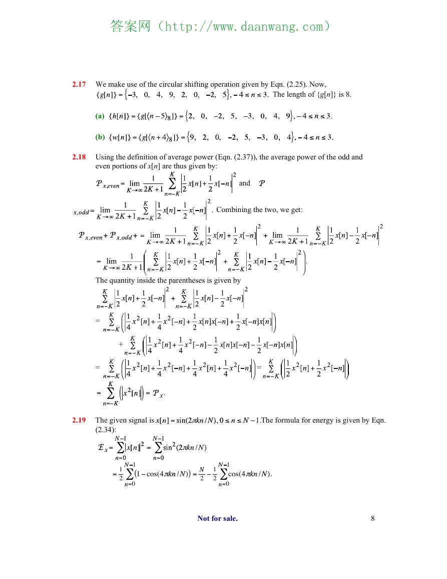
2.17 We make use of the circular shifting operation given by Eqn. (2.25). Now,
The length of {[]} is 8.
= {
}
(a)
(b)
=
=
+
= {
= {
}
}
2.18 Using the definition of average power (Eqn. (2.37)), the average power of the odd and
even portions of [] are thus given by:
=
+
=
+
and
Combining the two, we get:
The quantity inside the parentheses is given by
=
+
=
=
(
=
)
=
.
2.19 The given signal is
=
(2.34):
=
=
=
=
1
(
1 cos(4
=0
=
1
2
=
The formula for energy is given by Eqn.
/
)
)
=
2
1
2
1
cos(4
=0
/
)
.
Not for sale.
8
�




 2023年江西萍乡中考道德与法治真题及答案.doc
 2012年重庆南川中考生物真题及答案.doc
 2013年江西师范大学地理学综合及文艺理论基础考研真题.doc
 2020年四川甘孜小升初语文真题及答案I卷.doc
 2020年注册岩土工程师专业基础考试真题及答案.doc
 2023-2024学年福建省厦门市九年级上学期数学月考试题及答案.doc
 2021-2022学年辽宁省沈阳市大东区九年级上学期语文期末试题及答案.doc
 2022-2023学年北京东城区初三第一学期物理期末试卷及答案.doc
 2018上半年江西教师资格初中地理学科知识与教学能力真题及答案.doc
 2012年河北国家公务员申论考试真题及答案-省级.doc
 2020-2021学年江苏省扬州市江都区邵樊片九年级上学期数学第一次质量检测试题及答案.doc
 2022下半年黑龙江教师资格证中学综合素质真题及答案.doc