Extended Kalman Filter 入门讲义.pdf-资料库

grandpapatao-10462994-4744302543291167813.pdf-第1页.png

第1页 / 共7页

grandpapatao-10462994-4744302543291167813.pdf-第2页.png

第2页 / 共7页

grandpapatao-10462994-4744302543291167813.pdf-第3页.png

第3页 / 共7页

grandpapatao-10462994-4744302543291167813.pdf-第4页.png

第4页 / 共7页

grandpapatao-10462994-4744302543291167813.pdf-第5页.png

第5页 / 共7页

grandpapatao-10462994-4744302543291167813.pdf-第6页.png

第6页 / 共7页

grandpapatao-10462994-4744302543291167813.pdf-第7页.png

第7页 / 共7页

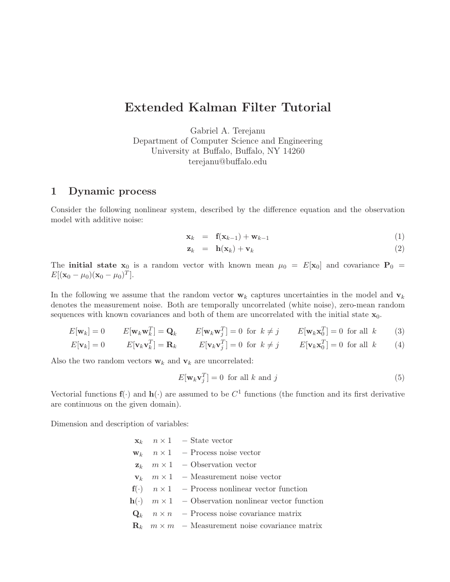
Extended Kalman Filter Tutorial Gabriel A. Terejanu Department of Computer Science and Engineering University at Buﬀalo, Buﬀalo, NY 14260 terejanu@buﬀalo.edu 1 Dynamic process Consider the following nonlinear system, described by the diﬀerence equation and the observation model with additive noise: xk = f(xk−1) + wk−1 zk = h(xk) + vk (1) (2) The initial state x0 is a random vector with known mean µ0 = E[x0] and covariance P0 = E[(x0 − µ0)(x0 − µ0)T ]. In the following we assume that the random vector wk captures uncertainties in the model and vk denotes the measurement noise. Both are temporally uncorrelated (white noise), zero-mean random sequences with known covariances and both of them are uncorrelated with the initial state x0. E[wk] = 0 E[vk] = 0 E[wkwT E[vkvT k ] = Qk k ] = Rk E[wkwT E[vkvT j ] = 0 for k 6= j j ] = 0 for k 6= j Also the two random vectors wk and vk are uncorrelated: E[wkvT j ] = 0 for all k and j E[wkxT E[vkxT 0 ] = 0 for all k 0 ] = 0 for all k (3) (4) (5) Vectorial functions f(·) and h(·) are assumed to be C 1 functions (the function and its ﬁrst derivative are continuous on the given domain). Dimension and description of variables: n × 1 − State vector xk n × 1 − Process noise vector wk zk m × 1 − Observation vector vk m × 1 − Measurement noise vector f(·) n × 1 − Process nonlinear vector function h(·) m × 1 − Observation nonlinear vector function n × n − Process noise covariance matrix Qk Rk m × m − Measurement noise covariance matrix

2 EKF derivation Assuming the nonlinearities in the dynamic and the observation model are smooth, we can expand f(xk) and h(xk) in Taylor Series and approximate this way the forecast and the next estimate of xk. Model Forecast Step Initially, since the only available information is the mean, µ0, and the covariance, P0, of the initial state then the initial optimal estimate xa 0 and error covariance is: xa 0 = µ0 = E[x0] P0 = E[(x0 − xa 0)(x0 − xa 0)T ] (6) (7) Assume now that we have an optimal estimate xa k − 1. The predictable part of xk is given by: k−1 ≡ E[xk−1|Zk−1] with Pk−1 covariance at time xf k ≡ E[xk|Zk−1] = E[f(xk−1) + wk−1|Zk−1] = E[f(xk−1)|Zk−1] Expanding f(·) in Taylor Series about xa k−1 we get: f(xk−1) ≡ f(xa k−1) + Jf(xa k−1)(xk−1 − xa k−1) + H.O.T. (8) (9) where Jf is the Jacobian of f(·) and the higher order terms (H.O.T.) are considered negligible. Hence, the Extended Kalman Filter is also called the First-Order Filter. The Jacobian is deﬁned as: Jf ≡   ∂f1 ∂x2 ∂f1 ∂x1 ... ∂fn ∂x1 ∂fn ∂x2 · · · . . . · · · ∂f1 ∂xn ... ∂fn ∂xn   where f(x) = (f1(x), f2(x), . . . , fn(x))T and x = (x1, x2, . . . , xn)T . The eq.(9) becomes: where ek−1 ≡ xk−1 − xa k−1. The expectated value of f(xk−1) conditioned by Zk−1: f(xk−1) ≈ f(xa k−1) + Jf(xa k−1)ek−1 E[f(xk−1)|Zk−1] ≈ f(xa k−1) + Jf(xa k−1)E[ek−1|Zk−1] where E[ek−1|Zk−1] = 0. Thus the forecast value of xk is: xf k ≈ f(xa k−1) Substituting (11) in the forecast error equation results: ef k ≡ xk − xf k = f(xk−1) + wk−1 − f(xa ≈ Jf(xa k−1)ek−1 + wk−1 k−1) 2 (10) (11) (12) (13) (14)

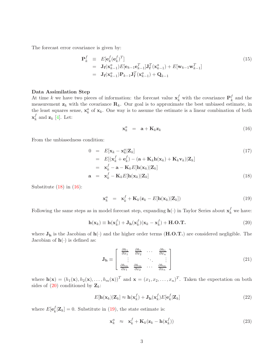
The forecast error covariance is given by: Pf k ≡ E[ef = Jf(xa = Jf(xa k )T ] k(ef k−1)E[ek−1eT k−1)Pk−1JT k−1]JT f (xa k−1) + E[wk−1wT k−1] f (xa k−1) + Qk−1 (15) Data Assimilation Step At time k we have two pieces of information: the forecast value xf k and the measurement zk with the covariance Rk. Our goal is to approximate the best unbiased estimate, in the least squares sense, xa k of xk. One way is to assume the estimate is a linear combination of both xf k and zk [4]. Let: k with the covariance Pf From the unbiasedness condition: xa k = a + Kkzk k|Zk] k) − (a + Kkh(xk) + Kkvk)|Zk] 0 = E[xk − xa k + ef = E[(xf = xf a = xf k − a − KkE[h(xk)|Zk] k − KkE[h(xk)|Zk] Substitute (18) in (16): k = xf xa k + Kk(zk − E[h(xk)|Zk]) (16) (17) (18) (19) Following the same steps as in model forecast step, expanding h(·) in Taylor Series about xf k we have: h(xk) ≡ h(xf k) + Jh(xf k)(xk − xf k) + H.O.T. (20) where Jh is the Jacobian of h(·) and the higher order terms (H.O.T.) are considered negligible. The Jacobian of h(·) is deﬁned as: Jh ≡   ∂h1 ∂x2 ∂h1 ∂x1 ... ∂hm ∂x1 ∂hm ∂x2 · · · . . . · · · ∂h1 ∂xn ... ∂hm ∂xn   (21) where h(x) = (h1(x), h2(x), . . . , hm(x))T and x = (x1, x2, . . . , xn)T . Taken the expectation on both sides of (20) conditioned by Zk: E[h(xk)|Zk] ≈ h(xf k) + Jh(xf k)E[ef k|Zk] where E[ef k |Zk] = 0. Substitute in (19), the state estimate is: k ≈ xf xa k + Kk(zk − h(xf k )) 3 (22) (23)

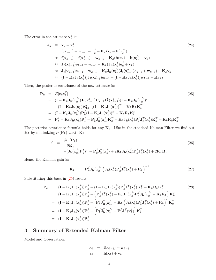
The error in the estimate xa k is: ek ≡ xk − xa k k − Kk(zk − h(xf k)) k−1) + wk−1 − Kk(h(xk) − h(xf k ) + vk) = f(xk−1) + wk−1 − xf ≈ f(xk−1) − f(xa ≈ Jf(xa ≈ Jf(xa ≈ (I − KkJh(xf k))Jf(xa k−1)ek−1 + wk−1 − Kk(Jh(xf k−1)ek−1 + wk−1 − KkJh(xf k)ef k)(Jf(xa k + vk) k−1)ek−1 + wk−1) − Kkvk k−1)ek−1 + (I − KkJh(xf k))wk−1 − Kkvk Then, the posterior covariance of the new estimate is: Pk ≡ E[ekeT k ] = (I − KkJh(xf +(I − KkJh(xf k))Jf(xa k−1)Pk−1JT f (xa k))Qk−1(I − KkJh(xf k−1)(I − KkJh(xf k))T + KkRkKT k k))T (24) (25) = (I − KkJh(xf k − KkJh(xf = Pf k))Pf k)Pf k(I − KkJh(xf k − Pf h (xf k JT k))T + KkRkKT k + KkJh(xf k)KT k k )Pf k JT h (xf k)KT k + KkRkKT k The posterior covariance formula holds for any Kk. Like in the standard Kalman Filter we ﬁnd out Kk by minimizing tr(Pk) w.r.t. Kk. 0 = ∂tr(Pk) ∂Kk = −(Jh(xf k)Pf k )T − Pf k JT h (xf k) + 2KkJh(xf k )Pf k JT h (xf k) + 2KkRk Hence the Kalman gain is: Kk = Pf k JT h (xf k )Jh(xf k )Pf k JT h (xf k) + Rk−1 Substituting this back in (25) results: Pk = (I − KkJh(xf = (I − KkJh(xf = (I − KkJh(xf = (I − KkJh(xf = (I − KkJh(xf k ))Pf k ))Pf k ))Pf k ))Pf k ))Pf k k JT k JT h (xf k))Pf k − (I − KkJh(xf k − Pf k − hPf k − hPf h (xf k ) − KkJh(xf k) − Kk Jh(xf h (xf k) − Pf k)KT k)Pf k JT k)Pf k)i KT h (xf h (xf k JT k JT k JT k k + KkRkKT k h (xf k) − KkRk KT k) + Rki KT k k k JT h (xf (26) (27) (28) 3 Summary of Extended Kalman Filter Model and Observation: xk = f(xk−1) + wk−1 zk = h(xk) + vk 4

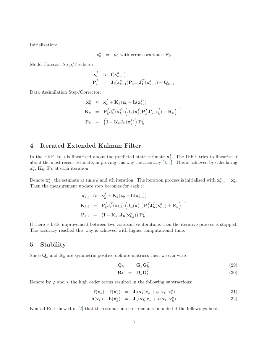
Initialization: Model Forecast Step/Predictor: xa 0 = µ0 with error covariance P0 xf k ≈ f(xa Pf k = Jf(xa k−1) k−1)Pk−1JT f (xa k−1) + Qk−1 Data Assimilation Step/Corrector: k + Kk(zk − h(xf k)Jh(xf k JT k ≈ xf xa Kk = Pf Pk = I − KkJh(xf k)) k)Pf k) Pf h (xf k k JT h (xf k) + Rk−1 4 Iterated Extended Kalman Filter In the EKF, h(·) is linearized about the predicted state estimate xf k . The IEKF tries to linearize it about the most recent estimate, improving this way the accuracy [3, 1]. This is achieved by calculating xa k, Kk, Pk at each iteration. Denote xa Then the measurement update step becomes for each i: k,i the estimate at time k and ith iteration. The iteration process is initialized with xa k,0 = xf k. k + Kk(zk − h(xa h (ˆxk,i)Jh(xa k JT k,i ≈ xf xa Kk,i = Pf Pk,i = I − Kk,iJh(xa k,i) Pf k,i)) k,i)Pf k k JT h (xa k,i) + Rk−1 If there is little improvement between two consecutive iterations then the iterative process is stopped. The accuracy reached this way is achieved with higher computational time. 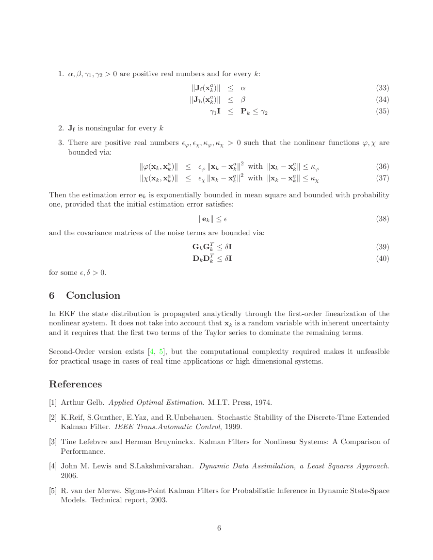5 Stability Since Qk and Rk are symmetric positive deﬁnite matrices then we can write: Qk = GkGT k Rk = DkDT k Denote by ϕ and χ the high order terms resulted in the following subtractions: f(xk) − f(xa h(xk) − h(xa k) = Jf(xa k) = Jh(xa k)ek + ϕ(xk, xa k) k)ek + χ(xk, xa k) Konrad Reif showed in [2] that the estimation error remains bounded if the followings hold: 5 (29) (30) (31) (32)

1. α, β, γ1, γ2 > 0 are positive real numbers and for every k: kJf(xa kJh(xa k)k ≤ α k)k ≤ β γ1I ≤ Pk ≤ γ2 (33) (34) (35) 2. Jf is nonsingular for every k 3. There are positive real numbers ǫϕ, ǫχ, κϕ, κχ > 0 such that the nonlinear functions ϕ, χ are bounded via: kϕ(xk, xa kχ(xk, xa k)k ≤ ǫϕ kxk − xa k)k ≤ ǫχ kxk − xa kk2 with kxk − xa kk2 with kxk − xa kk ≤ κϕ kk ≤ κχ (36) (37) Then the estimation error ek is exponentially bounded in mean square and bounded with probability one, provided that the initial estimation error satisﬁes: and the covariance matrices of the noise terms are bounded via: kekk ≤ ǫ GkGT DkDT k ≤ δI k ≤ δI (38) (39) (40) for some ǫ, δ > 0. 6 Conclusion In EKF the state distribution is propagated analytically through the ﬁrst-order linearization of the nonlinear system. It does not take into account that xk is a random variable with inherent uncertainty and it requires that the ﬁrst two terms of the Taylor series to dominate the remaining terms. Second-Order version exists [4, 5], but the computational complexity required makes it unfeasible for practical usage in cases of real time applications or high dimensional systems. References [1] Arthur Gelb. Applied Optimal Estimation. M.I.T. Press, 1974. [2] K.Reif, S.Gunther, E.Yaz, and R.Unbehauen. Stochastic Stability of the Discrete-Time Extended Kalman Filter. IEEE Trans.Automatic Control, 1999. [3] Tine Lefebvre and Herman Bruyninckx. Kalman Filters for Nonlinear Systems: A Comparison of Performance. [4] John M. Lewis and S.Lakshmivarahan. Dynamic Data Assimilation, a Least Squares Approach. 2006. [5] R. van der Merwe. Sigma-Point Kalman Filters for Probabilistic Inference in Dynamic State-Space Models. Technical report, 2003. 6

Figure 1: The block diagram for Extended Kalman Filter 7

资料库

Extended Kalman Filter 入门讲义.pdf

相关推荐

课程资源

热门标签

最新资料