Zero-inflated Negative Binomial Model and its Application in Car....pdf

发布时间：2022-05-30 发布人：admin 分类：说明书资料大小：0.56M 资料格式：pdf 举报版权申诉

weixin_38556189-12060468-16359647519208251438.pdf-第1页.png

第1页 / 共12页

weixin_38556189-12060468-16359647519208251438.pdf-第2页.png

第2页 / 共12页

weixin_38556189-12060468-16359647519208251438.pdf-第3页.png

第3页 / 共12页

weixin_38556189-12060468-16359647519208251438.pdf-第4页.png

第4页 / 共12页

weixin_38556189-12060468-16359647519208251438.pdf-第5页.png

第5页 / 共12页

weixin_38556189-12060468-16359647519208251438.pdf-第6页.png

第6页 / 共12页

weixin_38556189-12060468-16359647519208251438.pdf-第7页.png

第7页 / 共12页

weixin_38556189-12060468-16359647519208251438.pdf-第8页.png

第8页 / 共12页

文本预览

中国科技论文在线 http://www.paper.edu.cn Zero-inflated Negative Binomial Model and its Application in Car Insurance Jiang Tingting, Huang Wei** (College of Mathematics and Statistics of Chongqing University, Chongqing 401331) Abstract: Under many circumstances, most car insurance data appears to be zero-inflated and their risks are nonhomogeneous. These lead to general traditional claim frequency models lost their prediction effect, so they are unsuitable to fit this kind of data. This paper is using the car insurance data for GINB model, ZINB model and C-ZINB model to do empirical research, the results demonstrate that the C-ZINB model can overcome the risk of homogeneity and zero inflation very well. In addition, C-ZINB model has good simulation prediction effect. Key words: Statistics;Negative Binomial Distribution;Zero-inflated Model;Car Insurance 5 10 15 0 Introduction Relative to other financial industry, the insurance is a new type of financial industry. With the expansion of the various risks, the insurance is gradually developing into a global industry in just a few decades. Insurance usually can be divided into two categories: life insurance and non-life insurance. Life insurance has developed for a long time and had a lot of historical data, so scholars 20 have already get much achievement. Although formation of non-life insurance is earlier than life insurance, the study of non-life insurance is far later than life insurance. Therefore, the development of non-life insurance is slow and the historical data is less. Moreover, different insurance object obey different distribution. Even if we can determine what distribution the insurance object obeys, its parameter estimation is also very difficult. Sometimes, the loss 25 distribution of same risk also varies with time and environment. Because of the complexity of the loss factors, the scholars have difficulties making non-life insurance pricing. Generally speaking, non-life insurance is property insurance. In property insurance, the development of car insurance is most rapidly. With the development of economy, car becomes people’s main traffic tool. The increasing of the number of car is creating condition for the 30 development of car insurance. The birth of third-party liability insurance and mandatory traffic liability insurance is speeding up the development of car insurance too. Now, the proportion of car insurance in property insurance is the largest. The operating conditions of car insurance directly affect the economic benefits of property insurance company. Because of the rapid development of car insurance, how to stable the premiums and at the same 35 time reduce the loss ratios of car insurance is becoming the main problem. So the study of claim number of car insurance is particularly important. Secondly, because of deductible, no claims discount, personal factors and some other reasons, make insurant may not claim to the insurance company after the traffic accident. This lead to zero probability increases means spearing zero inflation. Therefore, how to solve the zero inflation becomes the major problem to actuaries. 40 This paper is modeling zero-inflated model with negative binomial distribution, and discussing the application of zero-inflated model in car insurance combined with the practical experience data. Brief author introduction:Jiang Tingting(1989-), female, Master, Main research: Statistical Methods and Application Correspondance author: Huang Wei(1968-), female, Associate Professor, Main research: Probability Statistics and Applications, Financial Engineering and Application, Stochastic Analysis and Application. E-mail: tan16.tt@163.com - 1 -

中国科技论文在线 1 Negative Binomial Model http://www.paper.edu.cn Negative binomial distribution not only can be satisfactorily used for fitting the claims data, but 45 also has a very simple property that its variance is greater than its mean. So it is good for fitting the actual data which is nonhomogeneous. Negative binomial distribution has been widely used in risk management because of this simple property. In early study, we generally assume that risk is homogeneous. The claim number obey the poisson distribution . It means in each risk is fixed and be a constant. But in practice, the 50 risk may not be homogeneity. Nonhomogeneous risk caused impossible be a constant. Let be the kind of risk’s random variable and probability distribution is as follow: . Then the , Assume that , then the probability density function of is: 55 Using the total probability formula, the probability distribution of the claim is given by: So obey the negative binomial distribution: . For , let , .Then the form of negative binomial 60 distribution becomes . The parameter means divergence parameter, the higher the , the more serious the risk of nonhomogeneous. And the probability density function is transformed as follow: （1） Its mean and variance are: 65 Let , then the negative binomial model is transformed into the generalized negative binomial model, namely GLNB model. - 2 - NPiNiiiNP1,2,,is,0,1,2!iiyiiiiiiPNyeyy,ii11iiife101!1111iiiiiiiiiiiyiiiiyiiPNyPNyfdeedyyyiN1,1iNNBiiiE22iiVark111,iikNNBkkkk1111111ikyiiiiiiiykkPNykkykiiEN1iiiVarNk01122expexp+iiiiippxxxx

中国科技论文在线 http://www.paper.edu.cn 70 the zero-inflated model is established by the generalized negative binomial model. means kinds of factor which affect the claim frequency. In this paper, 2 Zero-inflated Negative Binomial Model 2.1 Zero-inflated Model Zero-inflated model was first put forward by Johnson and Kotz[1]. They divide the source of count data into two parts: The first part explains the cause of zero inflation, and the count data can 75 only be zero. The second part is subject to a discrete distribution, the count data can be zero or a positive integer. It means the zero count process is a mixed probability distribution, the probability of zero comes from two parts: structural zero and sample zero. Let the random variable of claim frequency be , structural zero be , then the zero-inflated model is: 80 (2) Among it, the random variable is subject to a discrete distribution. The mean and variance of are: 85 2.2 Zero-inflated Negative Binomial Model Let the random variable of formula (2) obey the negative binomial distribution which means , then the zero-inflated model is transformed into zero-inflated negative binomial model: 90 Its mean and variance are: （3） Under normal circumstances, structural zero be a constant, In order to ensure , we usually let: 95 （4） - 3 - 12,,,iiipxxxixp1,,iYis01(1)(1)1,2iiiiiiiiiiPYyPKyy=0PYyPKyy=，，，iKiY(1)iiEYEK2()(1)()iiiVarYEKkEKiK111,iikKNBkk111111111(1)(1)1,21ikiiiikyiiiiiiiikPYyy=0kykkPYyy=kkyk，，，1iiEY21iiiVarYk01logln1ita

中国科技论文在线 http://www.paper.edu.cn Solution of this equation is . Take it into formula (3), it is known as the ZINB model: （5） Generally, we use the maximum likelihood estimation method to estimate ZINB model’s 100 parameters. Due to the logarithmic likelihood function of ZINB model is nonlinear, so it needs to use the numerical iteration method. The logarithmic likelihood function of ZINB model can be expressed as: Using the logarithm likelihood function and numerical iteration method, the parameter estimation 105 can be determined. 2.3 C-ZINB model As mentioned above, various factors influence zero probability. In practical problems, the abnormal zero probability is generally not only caused by single factor, it also may be caused by a number of factors. So it seems not very reasonable if assume as a constant. Now, on the basis of 110 the ZINB model, transform formula (4) as follows: Among it, , means kinds of factor which affect the zero probability. Then the formula (5) is transformed into the C-ZINB model: 115 3 Empirical Research 3.1 Model Select Criteria In this paper, we compare models’ fitting effect according to the following principles. - 4 - exp1expaa11111111111111,211ikaiiiaaikyiiiiiaiiiekPYyy=0eekykkPYyy=ekkyk，，，101101lnln1ln1ln1lnln!lnln1iiikaaiyyiiiiiiyrlLneekkrykyykykklogln1iiiiiitaz01122+ziiiimmzzz12,,,iiiimzzzzm11111111111111,211iiiiikziiizzikyiiiiiziiiekPYyy=0eekykkPYyy=ekkyk，，，

中国科技论文在线 3.1.1 Akaike Information Criterion (AIC) http://www.paper.edu.cn 120 Akaike information criterion is created by Japanese statistician Akaike[2]. It can eatimate the complexity and superiority of model. The formula of AIC is as follow: is the logarithmic likelihood function value of model, is the number of parameters. Akaike suggests that the best model has the smallest AIC value. 125 3.1.2 Bayesian Information Criterion (BIC) Schwarz[3] created bayesian information criterion on the basis of AIC. BIC is established under the bayesian formula, its formula is as follow: is the logarithmic likelihood function value of model, is the number of parameters. is the 130 sample size. Like the AIC, the smaller the BIC value is, the beat the model is. But the difference is that the BIC considers the effect of sample size. 3.1.3 Vuong Test Vuong test can be used to estimate the goodness of fit between the non-nested models. Firstly let: 135 means the sample’s predicted probability of the model. Then the Vuong test statistics of model 1 relative to model 2 can be defined as: In this formula, , , statistics obeys normal distribution. 140 Vuong[4] have proved that, Model 1 is better than model 2 while ; Model 2 is better than model 1 while ; but it cannot judge while . 3.2 Data Description In order to do research with car insurance, the data comes from “Generalized Linear Models for Insurance Data” which is third party liability insurance of Australia. It contains 10303 samples. 145 The statistical description of claim frequency and the frequency distribution are as follow: Tab. 1 Statistical description of the claim counts Variable Name Mean Claim Counts 0.80 150 MAX 5 MIN 0 Std. 1.15 - 5 - 22AIClplp2lnBIClpnlpn12lniiiiiPYXmPYXjiiPYXijmnmVS11niimmn211nmiiSmmnV1.96V1.96V1.96V

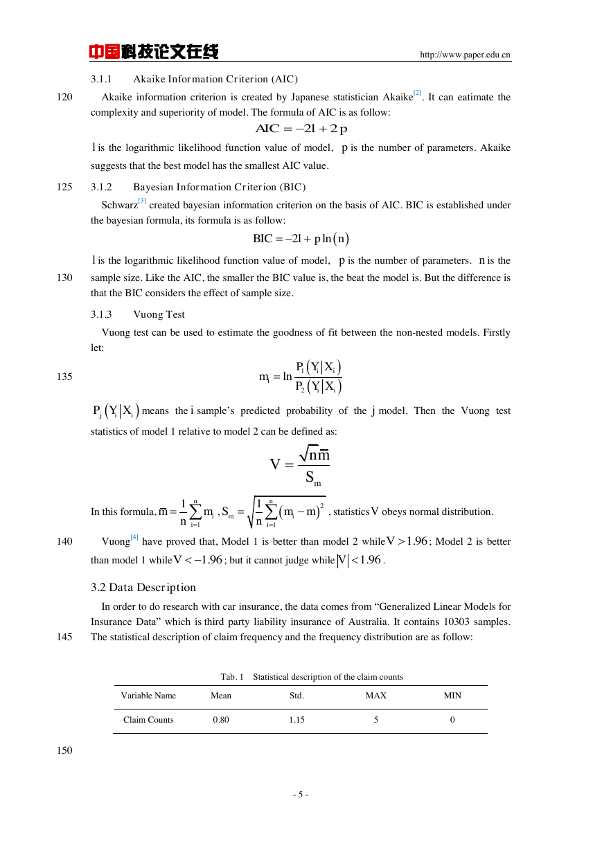
中国科技论文在线 http://www.paper.edu.cn Tab. 2 Frequency of the claim counts Claim Counts Frequency Frequency Cumulative Frequency 0 1 2 3 4 5 6293 1279 1492 992 225 22 0.6108 0.1241 0.1448 0.0963 0.0219 0.0021 0.6108 0.7349 0.8797 0.9760 0.9979 1.0000 155 160 Fig. 1 Histogram of the claim frequency It can be seen that the claim number of zero is bigger, the proportion of zero accounts for 62.08%. Using the traditional poisson distribution and negative binomial distribution to fit claim 165 frequency will lead the results appeared deviation. The fitting results of traditional poisson distribution and negative binomial distribution are as follow: - 6 -

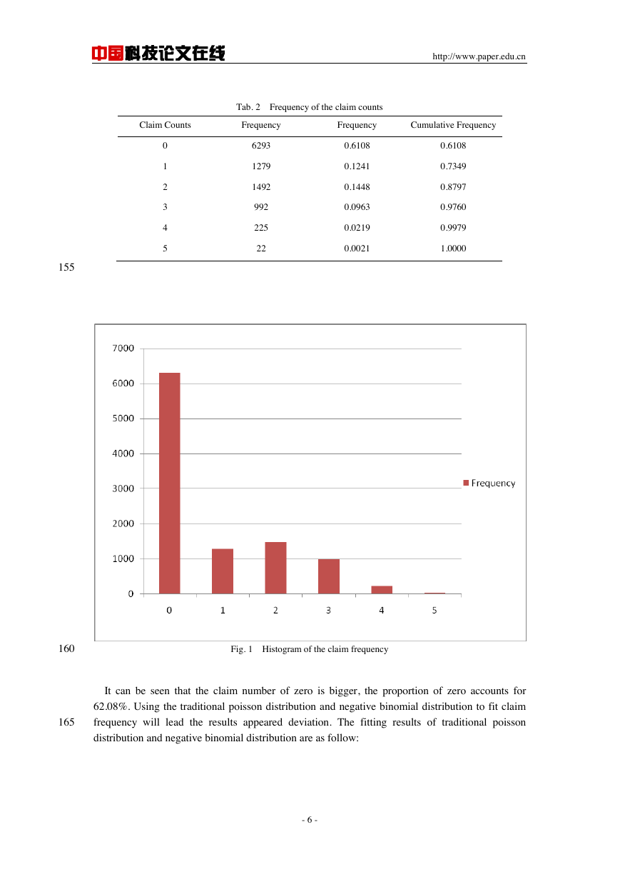
中国科技论文在线 http://www.paper.edu.cn 170 Tab. 3 Fitting result with poisson and negative binomial distribution Claim Counts Original Frequency Poisson Negative Binomial 0 1 2 3 4 5 6293 1279 1492 992 225 22 4626 3704 1483 396 79 13 6194 2470 985 393 157 62 175 Fig. 2 Contrast of fitting results In table 3, the fitting effect of poisson distribution is worse than negative binomial distribution. 180 It means the risk of data is nonhomogeneous. Then observe figure 2, we find that even the negative binomial distribution cannot get satisfying fitting results. Now, we use generalized negative binomial model and zero-inflated model to fit claim frequency. According to the influence factors of car, this paper we select age, gender, marital status, educational background, type of car, car use, driving area and insurance period as the research 185 objects. Assign the influence factors and the statistical description of them are as follow: - 7 -

中国科技论文在线 http://www.paper.edu.cn 190 Tab. 4 Variable assignment of influencing factors Influence Factors Variable Name Age Gender Marital Status Age Gender Married Variable Assignment Measurement Data Male=1, Female=0 Single=1, Married=0 Educational Background Education Below High School=0, High school or above=1 Type of Car Car Use Driving Area Insurance Period Type Use Area Years Sports Car=1, Sedan=2, SUV=3, Pickup=4, Panel Truck=5, Van=6 Private=1, Commercial=0 Suburb=1, Urban=0 Measurement Data Tab. 5 Statistical description of the quantitative index Variable Name Age Years Mean 44.84 5.33 Std. 8.61 4.11 MAX 81 25 MIN 16 1 195 Tab. 6 Statistical description of the qualitative index Variable Name Gender Married Education Type Use Area Frequency Proportion(%) Frequency Proportion(%) Classification of cases Male（4758） Single（4114） Below High School(1511) Sports Car（1179） SUV（2883） Panel Truck（853） Private（6513） Suburb（4631） 46.18 39.93 14.70 11.44 27.98 8.28 63.21 44.95 Female（5545） Married（6189） High school or above（8788） Sedan（2694） Pickup（1772） Van（922） Commercial（3790） Urban（5672） 53.82 60.07 85.30 26.15 17.20 8.95 36.79 55.05 3.3 Model Simulation 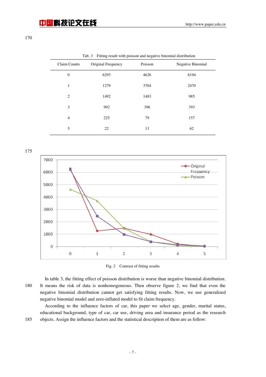According to the above information, we fit claim data with GLNB model, ZINB model and C-ZINB model. We choose the eight factors as the negative binomial’s covariate in all models in order to comprehensive analyze. And we choose the eight factors as the structural zero’s covariate 200 Too. The fitting results are as follow: Tab. 7 Fitting results Parameter Estimation Intercept GLNB Negative Binomial 0.1259 （0.1069)* ZINB Negative Binomial 0.5705 (0.0835)* C-ZINB Negative Binomial Structural Zero 0.3758 -0.9039 （0.0918）* （0.1783）* - 8 -

分享到：

赞收藏

资料库

Zero-inflated Negative Binomial Model and its Application in Car....pdf

相关推荐

开发技术

热门标签

最新资料