An Online Algorithm for Segmenting Time Series
Selina Chu
David Hart
Michael Pazzani
Eamonn Keogh
Department of Information and Computer Science
University of California, Irvine, California 92697 USA
{eamonn, selina, dhart, pazzani}@ics.uci.edu
Abstract
In recent years, there has been an explosion of interest in mining time series databases. As with most
computer science problems, representation of the data is the key to efficient and effective solutions. One of
the most commonly used representations is piecewise linear approximation. This representation has been
used by various researchers to support clustering, classification, indexing and association rule mining of
time series data. A variety of algorithms have been proposed to obtain this representation, with several
algorithms having been independently rediscovered several times. In this paper, we undertake the first
extensive review and empirical comparison of all proposed techniques. We show that all these algorithms
have fatal flaws from a data mining perspective. We introduce a novel algorithm that we empirically show
to be superior to all others in the literature.
1. Introduction
In recent years, there has been an explosion of interest in mining time series databases. As with
most computer science problems, representation of the data is the key to efficient and effective
solutions. Several high level representations of time series have been proposed, including Fourier
Transforms [1,13], Wavelets [4], Symbolic Mappings [2, 5, 24] and Piecewise Linear
Representation (PLR). In this work, we confine our attention to PLR, perhaps the most frequently
used representation [8, 10, 12, 14, 15, 16, 17, 18, 20, 21, 22, 25, 27, 28, 30, 31].
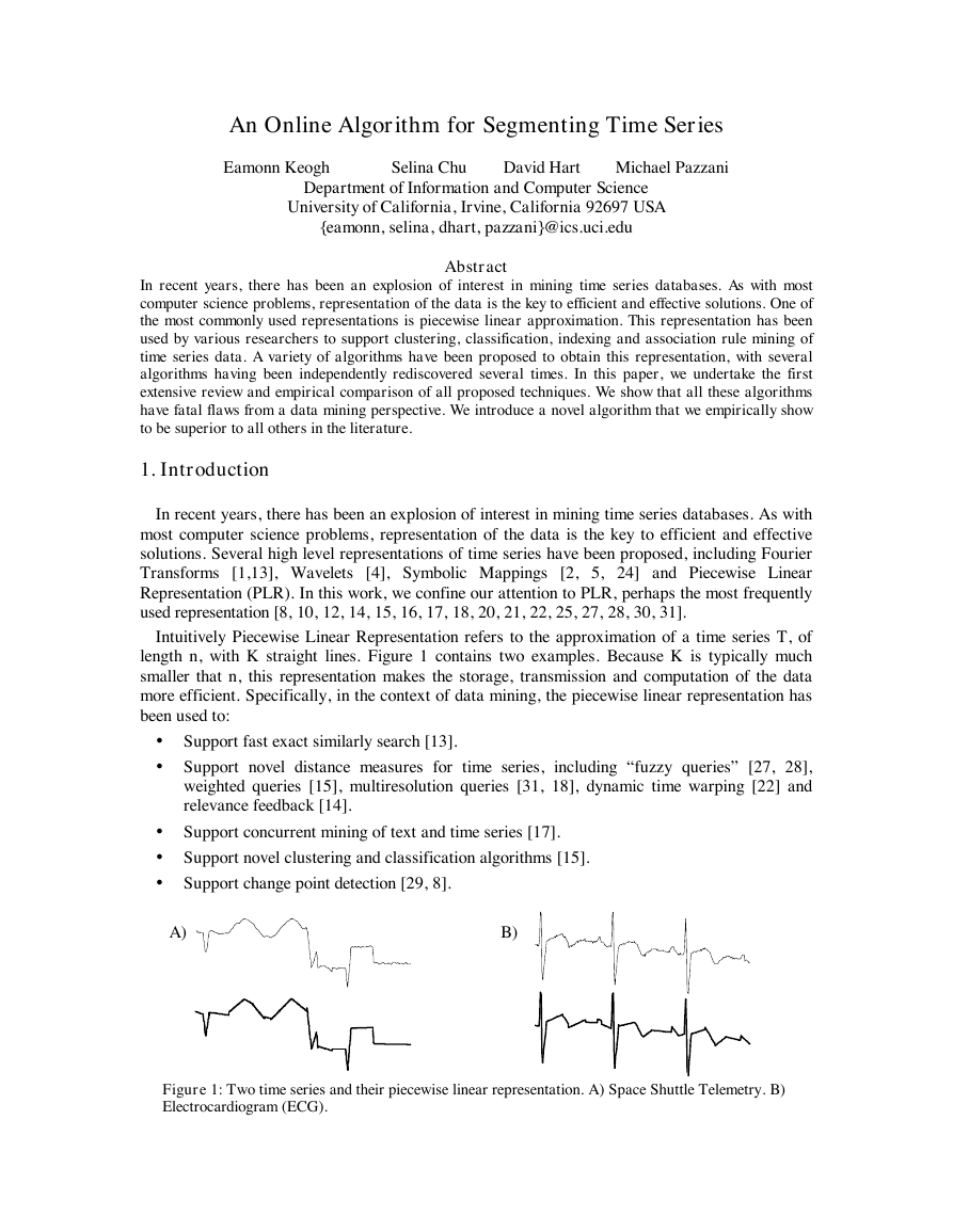
Intuitively Piecewise Linear Representation refers to the approximation of a time series T, of
length n, with K straight lines. Figure 1 contains two examples. Because K is typically much
smaller that n, this representation makes the storage, transmission and computation of the data
more efficient. Specifically, in the context of data mining, the piecewise linear representation has
been used to:
• Support fast exact similarly search [13].
• Support novel distance measures for time series, including “fuzzy queries” [27, 28],
weighted queries [15], multiresolution queries [31, 18], dynamic time warping [22] and
relevance feedback [14].
• Support concurrent mining of text and time series [17].
• Support novel clustering and classification algorithms [15].
• Support change point detection [29, 8].
A)
B)
Figure 1: Two time series and their piecewise linear representation. A) Space Shuttle Telemetry. B)
Electrocardiogram (ECG).
�
Surprisingly, in spite of the ubiquity of this representation, with the exception of [27], there has
been little attempt to understand and compare the algorithms that produce it. Indeed, there does
not even appear to be a consensus on what to call such an algorithm. For clarity, we will refer to
these types of algorithm, which input a time series and return a piecewise linear representation, as
segmentation algorithms.
The segmentation problem can be framed in several ways.
• Given a time series T, produce the best representation using only K segments.
• Given a time series T, produce the best representation such that the maximum error for any
segment does not exceed some user-specified threshold, max_error.
• Given a time series T, produce the best representation such that the combined error of all
segments is less than some user-specified threshold, total_max_error.
As we shall see in later sections, not all algorithms can support all these specifications.
Segmentation algorithms can also be classified as batch or online. This is an important
distinction because many data mining problems are inherently dynamic [30, 12].
Data mining researchers, who needed to produce a piecewise linear approximation, have
typically either independently rediscovered an algorithm or used an approach suggested in related
literature. For example, from the fields of cartography or computer graphics [6, 9, 26].
In this paper, we review the three major segmentation approaches in the literature and provide
an extensive empirical evaluation on a very heterogeneous collection of datasets from finance,
medicine, manufacturing and science. The major result of these experiments is that that only
online algorithm in the literature produces very poor approximations of the data, and that the only
algorithm that consistently produces high quality results and scales linearly in the size of the data
is a batch algorithm. These results motivated us to introduce a new algorithm that scales linearly
in the size of the data set, is online, and produces high quality approximations.
The rest of the paper is organized as follows. In Section 2, we provide an extensive review of
the algorithms in the literature. We explain the basic approaches, and the various modifications
and extensions by data miners. In Section 3, we provide a detailed empirical comparison of all the
algorithms. We will show that the most popular algorithms used by data miners can in fact
produce very poor approximations of the data. The results will be used to motivate the need for a
new algorithm that we will introduce and validate in Section 4. Section 5 offers conclusions and
directions for future work.
2. Background and Related Work
In this section, we describe the three major approaches to time series segmentation in detail.
Almost all the algorithms have 2 and 3 dimensional analogues, which ironically seem to be better
understood. A discussion of the higher dimensional cases is beyond the scope of this paper. We
refer the interested reader to [9], which contains an excellent survey.
Although appearing under different names and with slightly different implementation details,
most time series segmentation algorithms can be grouped into one of the following three
categories.
• Sliding Windows: A segment is grown until it exceeds some error bound. The process
repeats with the next data point not included in the newly approximated segment.
• Top-Down: The time series is recursively partitioned until some stopping criteria is met.
• Bottom-Up: Starting from the finest possible approximation, segments are merged until
some stopping criteria is met.
�
Table 1 contains the notation used in this paper.
T
T[a:b]
Seg_TS
create_segment(T)
calculate_error(T)
A time series in the form t1,t2,…,t n
The subsection of T from a to b, ta,ta+1,…,t b
A piecewise linear approximation of a time series of length n with K
segments. Individual segments can be addressed with Seg_TS(i).
A function which takes in a time series and returns a linear segment
approximation of it.
A function which takes in a time series and returns the approximation
error of the linear segment approximation of it.
Table 1: The notation used in this paper
Given that we are going to approximate a time series with straight lines, there are at least two
ways we can find the approximating line.
• Linear Interpolation: Here the approximating line for the subsequence T[a:b] is simply
the line connecting ta and tb. This can be obtained in constant time.
• Linear Regression: Here the approximating line for the subsequence T[a:b] is taken to be
the best fitting line in the least squares sense [27]. This can be obtained in time linear in the
length of segment.
The two techniques are illustrated in Figure 2. Linear interpolation tends to closely align the
endpoint of consecutive segments, giving the piecewise approximation a “smooth” look. In
contrast, piecewise linear regression can produce a very disjointed look on some datasets. The
aesthetic superiority of linear interpolation, together with its low computational complexity has
made it the technique of choice in computer graphic applications [9]. However, the quality of the
approximating line, in terms of Euclidean distance, is generally inferior to the regression
approach.
Linear
Interpolation
Linear
Regression
Figure 2: Two 10-segment approximations of electrocardiogram data. The approximation created
using linear interpolation has a smooth aesthetically appealing appearance because all the endpoints
of the segments are aligned. Linear regression, in contrast, produces a slightly disjointed appearance
but a tighter approximation in terms of residual error.
In this paper, we deliberately keep our descriptions of algorithms at a high level, so that either
technique can be imagined as the approximation technique. In particular, the pseudocode function
create_segment(T)can be imagined as using interpolation, regression or any other
technique.
All segmentation algorithms also need some method to evaluate the quality of fit for a potential
segment. A measure commonly used in conjunction with linear regression is the sum of squares,
or the residual error. This is calculated by taking all the vertical differences between the best-fit
line and the actual data points, squaring them and then summing them together. Another
commonly used measure of goodness of fit is the distance between the best fit line and the data
point furthest away in the vertical direction (i.e. the L¥ norm between the line and the data). As
before, we have kept our descriptions of the algorithms general enough to encompass any error
�
measure. In particular, the pseudocode function calculate_error(T)can be imagined as
using any sum of squares, furthest point, or any other measure.
2.1 The Sliding Window Algorithm.
The Sliding Window algorithm works by anchoring the left point of a potential segment at the
first data point of a time series, then attempting to approximate the data to the right with
increasing longer segments. At some point i, the error for the potential segment is greater than the
user-specified threshold, so the subsequence from the anchor to i-1 is transformed into a segment.
The anchor is moved to location i, and the process repeats until the entire time series has been
transformed into a piecewise linear approximation. The pseudocode for the algorithm is shown in
Table 2.
Algorithm Seg_TS = Sliding_Window(T , max_error)
anchor = 1;
while not finished segmenting time series
i = 2;
while calculate_error(T[anchor: anchor + i ]) < max_error
end;
Seg_TS = concat(Seg_TS, create_segment(T[anchor: anchor + (i-1)]);
anchor = anchor + i;
i = i + 1;
end;
Table 2: The generic Sliding Window algorithm
The Sliding Window algorithm is attractive because of its great simplicity, intuitiveness and
particularly the fact that it is an online algorithm. Several variations and optimizations of the
basic algorithm have been proposed. Koski et al. noted that on ECG data it is possible to speed up
the algorithm by incrementing the variable i by “leaps of length k” instead of 1. For k = 15 (at
400Hz), the algorithm is 15 times faster with little effect on the output [12].
Depending on the error measure used, there may be other optimizations possible. Vullings et al.
noted that since the residual error is monotonically non-decreasing with the addition of more data
points, one does not have to test every value of i from 2 to the final chosen value [30]. They
suggest initially setting i to s, where s is the mean length of the previous segments. If the guess
was pessimistic (the measured error is still less than max_error) then the algorithm continues
to increment i as in the classic algorithm. Otherwise they begin to decrement i until the measured
error is less than max_error. This optimization can greatly speed up the algorithm if the mean
length of segments is large in relation to the standard deviation of their length. The monotonically
non-decreasing property of residual error also allows binary search for the length of the segment.
Surprisingly, no one we are aware of has suggested this.
The Sliding Window algorithm can give pathologically poor results under some circumstances.
Most researchers have not reported this [25, 31], perhaps because they tested the algorithm on
stock market data, and its relative performance is best on noisy data. Shatkay (1995), in contrast,
does notice the problem and gives elegant examples and explanations [27]. They consider three
variants of the basic algorithm, each designed to be robust to a certain case, but they underline the
difficulty of producing a single variant of the algorithm which is robust to arbitrary data sources.
Park et al. (2001) suggested modifying the algorithm to create “monotonically changing”
t2‡
tn. This modification worked well on the smooth synthetic dataset it was demonstrated on.
segments [21]. That is, all segments consist of data points of the form of t1 £
… ‡
tn or t1 ‡
… £
t2£
�
But on real world datasets with any amount of noise, the approximation is greatly
overfragmented.
Variations on the Sliding Window algorithm are particularly popular with the medical
community (where it is known as FAN or SAPA), since patient monitoring is inherently an online
task [11, 12, 19, 30].
2.2 The Top-Down Algorithm.
The Top-Down algorithm works by considering every possible partitioning of the times series
and splitting it at the best location. Both subsections are then tested to see if their approximation
error is below some user-specified threshold. If not, the algorithm recursively continues to split
the subsequences until all the segments have approximation errors below the threshold. The
pseudocode for the algorithm is shown in Table 3.
Algorithm Seg_TS = Top_Down(T , max_error)
best_so_far = inf;
for i = 2 to length(T) - 2 // Find best place to split the time series.
improvement_in_approximation = improvement_splitting_here(T,i);
if improvement_in_approximation < best_so_far
breakpoint = i;
best_so_far = improvement_in_approximation;
end;
end;
// Recursively split the left segment if necessary.
if calculate_error(T[1:breakpoint]) > max_error
Seg_TS = Top_Down(T[1: breakpoint]);
end;
// Recursively split the right segment if necessary.
if calculate_error( T[breakpoint + 1:length(T)] ) > max_error
Seg_TS = Top_Down(T[breakpoint + 1: length(T)]);
end;
Table 3: The generic Top-Down algorithm
Variations on the Top-Down algorithm (including the 2-dimensional case) were independently
introduced in several fields in the early 1970’s. In cartography, it is known as the Douglas-
Peucker algorithm [6]; in image processing, it is known as Ramers algorithm [26]. Most
researchers in the machine learning/data mining community are introduced to the algorithm in the
classic textbook by Duda and Harts, which calls it “Iterative End-Points Fits”[7].
In the data mining community, the algorithm has been used by [18] to support a framework for
mining sequence databases at multiple abstraction levels. Shatkay and Zdonik use it (after
considering alternatives such as Sliding Windows) to support approximate queries in time series
databases [28].
Park et al. introduced a modification where they first perform a scan over the entire dataset
marking every peak and valley [22]. These extreme points is used to create an initial
segmentation, and the Top-Down algorithm is applied to each of the segments (in case the error
on an individual segment was still too high). They then use the segmentation to support a special
case of dynamic time warping. This modification worked well on the smooth synthetic dataset it
�
was demonstrated on. But on real world data sets with any amount of noise, the approximation is
greatly overfragmented.
Lavrenko et al. uses the Top-Down algorithm to support the concurrent mining of text and
time series [17]. They attempt to discover the influence of news stories on financial markets.
Their algorithm contains some interesting modifications including a novel stopping criteria based
on the t-test.
Finally Smyth and Ge use the algorithm to produce a representation which can support a
Hidden Markov Model approach to both change point detection and pattern matching [8].
2.3 The Bottom-Up Algorithm.
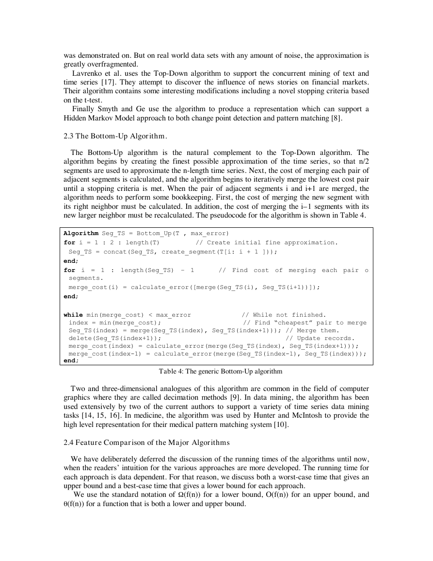
The Bottom-Up algorithm is the natural complement to the Top-Down algorithm. The
algorithm begins by creating the finest possible approximation of the time series, so that n/2
segments are used to approximate the n-length time series. Next, the cost of merging each pair of
adjacent segments is calculated, and the algorithm begins to iteratively merge the lowest cost pair
until a stopping criteria is met. When the pair of adjacent segments i and i+1 are merged, the
algorithm needs to perform some bookkeeping. First, the cost of merging the new segment with
its right neighbor must be calculated. In addition, the cost of merging the i–1 segments with its
new larger neighbor must be recalculated. The pseudocode for the algorithm is shown in Table 4.
Algorithm Seg_TS = Bottom_Up(T , max_error)
for i = 1 : 2 : length(T) // Create initial fine approximation.
Seg_TS = concat(Seg_TS, create_segment(T[i: i + 1 ]));
end;
for i = 1 : length(Seg_TS) – 1 // Find cost of merging each pair of
segments.
merge_cost(i) = calculate_error([merge(Seg_TS(i), Seg_TS(i+1))]);
end;
while min(merge_cost) < max_error // While not finished.
index = min(merge_cost); // Find “cheapest” pair to merge.
Seg_TS(index) = merge(Seg_TS(index), Seg_TS(index+1))); // Merge them.
delete(Seg_TS(index+1)); // Update records.
merge_cost(index) = calculate_error(merge(Seg_TS(index), Seg_TS(index+1)));
merge_cost(index-1) = calculate_error(merge(Seg_TS(index-1), Seg_TS(index)));
end;
Table 4: The generic Bottom-Up algorithm
Two and three-dimensional analogues of this algorithm are common in the field of computer
graphics where they are called decimation methods [9]. In data mining, the algorithm has been
used extensively by two of the current authors to support a variety of time series data mining
tasks [14, 15, 16]. In medicine, the algorithm was used by Hunter and McIntosh to provide the
high level representation for their medical pattern matching system [10].
2.4 Feature Comparison of the Major Algorithms
We have deliberately deferred the discussion of the running times of the algorithms until now,
when the readers’ intuition for the various approaches are more developed. The running time for
each approach is data dependent. For that reason, we discuss both a worst-case time that gives an
upper bound and a best-case time that gives a lower bound for each approach.
We use the standard notation of W
(f(n)) for a lower bound, O(f(n)) for an upper bound, and
q(f(n)) for a function that is both a lower and upper bound.
�
Definitions and Assumptions. The number of data points is n, the number of segments we plan
to create is K, and thus the average segment length is L = n/K. The actual length of segments
created by an algorithm varies and we will refer to the lengths as Li.
All algorithms, except top-down, perform considerably worse if we allow any of the Li to
become very large (say n/4), so we assume that the algorithms limit each Li to some multiple cL
of the average length. It is trivial to code the algorithms to enforce this, so the time analysis that
follows is exact when the algorithm includes this limit.
All algorithms, except top-down, perform considerably worse if we allow any of the Li to
become very large (say n/4), so we assume that the algorithms limit the maximum length L to
some multiple of the average length. It is trivial to code the algorithms to enforce this, so the time
analysis that follows is exact when the algorithm includes this limit. Empirical results show,
however, that the segments generated (with no limit on length) are tightly clustered around the
average length, so this limit has little effect in practice.
We assume that for each set S of points, we compute a best segment and compute the error in
q(n) time. This reflects the way these algorithms are coded in practice, which is to use a packaged
algorithm or function to do linear regression. We note, however, that we believe one can produce
asymptotically faster algorithms if one custom codes linear regression (or other best fit
algorithms) to reuse computed values so that the computation is done in less than O(n) time in
subsequent steps. We leave that as a topic for future work. In what follows, all computations of
best segment and error are assumed to be q(n).
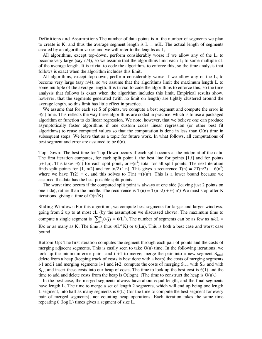
Top-Down: The best time for Top-Down occurs if each split occurs at the midpoint of the data.
The first iteration computes, for each split point i, the best line for points [1,i] and for points
[i+1,n]. This takes q (n) for each split point, or q(n2) total for all split points. The next iteration
finds split points for [1, n/2] and for [n/2+1,n]. This gives a recurrence T(n) = 2T(n/2) + q(n2)
where we have T(2) = c, and this solves to T(n) =W
(n2). This is a lower bound because we
assumed the data has the best possible split points.
The worst time occurs if the computed split point is always at one side (leaving just 2 points on
one side), rather than the middle. The recurrence is T(n) = T(n -2) + q( n2) We must stop after K
iterations, giving a time of O(n2K).
Sliding Windows: For this algorithm, we compute best segments for larger and larger windows,
going from 2 up to at most cL (by the assumption we discussed above). The maximum time to
compute a single segment is
)(q = q (L2). The number of segments can be as few as n/cL =
K/c or as many as K. The time is thus q(L2 K) or q(Ln). This is both a best case and worst case
bound.
cL
=
i
i
2
Bottom Up: The first iteration computes the segment through each pair of points and the costs of
merging adjacent segments. This is easily seen to take O(n) time. In the following iterations, we
look up the minimum error pair i and i +1 to merge; merge the pair into a new segment Snew;
delete from a heap (keeping track of costs is best done with a heap) the costs of merging segments
i-1 and i and merging segments i+1 and i+2; compute the costs of merging Snew with Si-1 and with
Si-2; and insert these costs into our heap of costs. The time to look up the best cost is q(1) and the
time to add and delete costs from the heap is O(logn). (The time to construct the heap is O(n).)
In the best case, the merged segments always have about equal length, and the final segments
have length L. The time to merge a set of length 2 segments, which will end up being one length
L segment, into half as many segments is q(L) (for the time to compute the best segment for every
pair of merged segments), not counting heap operations. Each iteration takes the same time
repeating q (log L) times gives a segment of size L.
�
The number of times we produce length L segments is K, so the total time is W
(K L log L) =
(n log n/K). The heap operations may take as much as O(nlogn). For a lower bound we have
proven just W
(n log n/K ).
In the worst case, the merges always involve a short and long segment, and the final segments
are mostly of length cL. The time to compute the cost of merging a length 2 segment with a
length i segment is q(i), and the time to reach a length cL segment is
)(q = q(L2). There are
at most n/cL such segments to compute, so the time is n/cL * q(L2) = O(Ln). (Time for heap
operations is inconsequential.)
cL
=
i
i
2
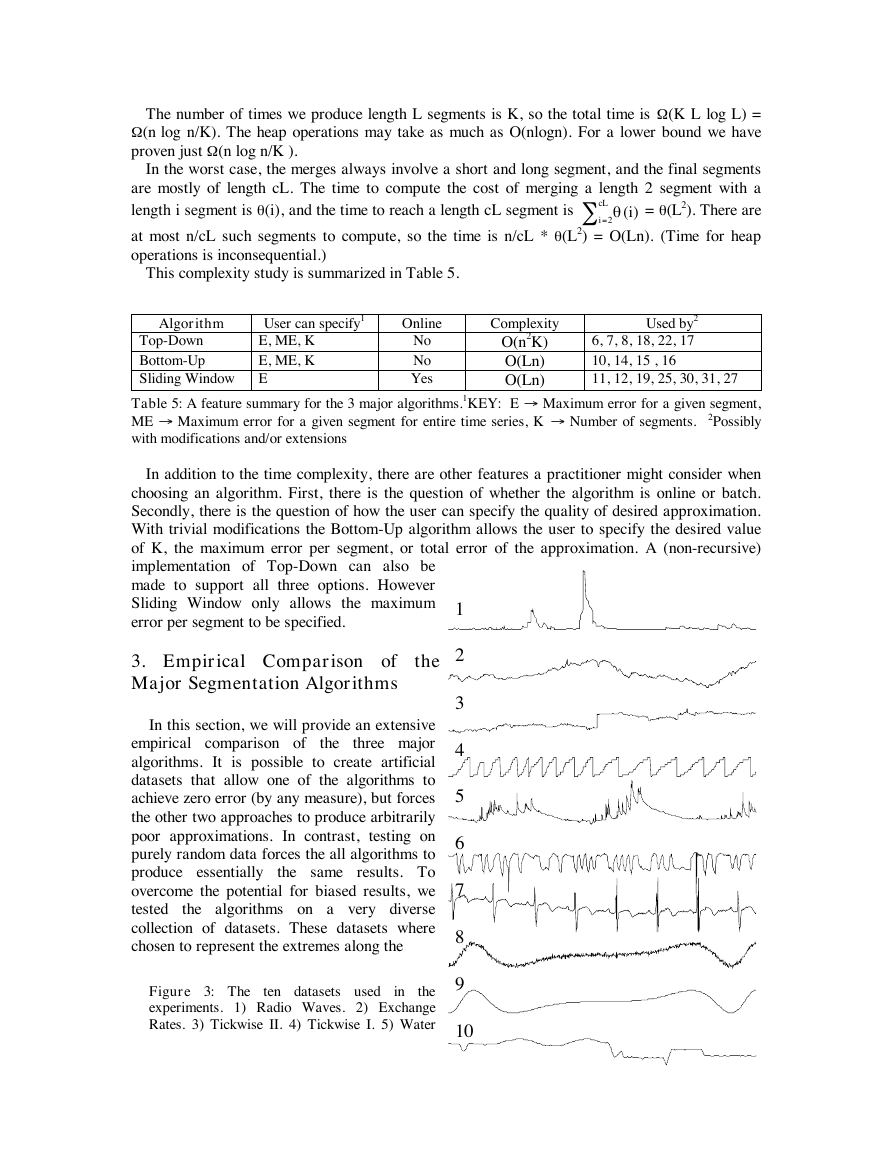
This complexity study is summarized in Table 5.
Online
Algorithm
User can specify1
E, ME, K
E, ME, K
E
Top-Down
Bottom-Up
Sliding Window
Table 5: A feature summary for the 3 major algorithms.1KEY: E fi
ME fi
with modifications and/or extensions
Maximum error for a given segment for entire time series, K fi
O(n2K)
O(Ln)
O(Ln)
No
No
Yes
Complexity
Used by2
6, 7, 8, 18, 22, 17
10, 14, 15 , 16
11, 12, 19, 25, 30, 31, 27
Maximum error for a given segment,
Number of segments. 2Possibly
In addition to the time complexity, there are other features a practitioner might consider when
choosing an algorithm. First, there is the question of whether the algorithm is online or batch.
Secondly, there is the question of how the user can specify the quality of desired approximation.
With trivial modifications the Bottom-Up algorithm allows the user to specify the desired value
of K, the maximum error per segment, or total error of the approximation. A (non-recursive)
implementation of Top-Down can also be
made to support all three options. However
Sliding Window only allows the maximum
error per segment to be specified.
1
3. Empirical Comparison of the
Major Segmentation Algorithms
the
In this section, we will provide an extensive
empirical comparison of
three major
algorithms. It is possible to create artificial
datasets that allow one of the algorithms to
achieve zero error (by any measure), but forces
the other two approaches to produce arbitrarily
poor approximations. In contrast, testing on
purely random data forces the all algorithms to
produce essentially
the same results. To
overcome the potential for biased results, we
tested
the algorithms on a very diverse
collection of datasets. These datasets where
chosen to represent the extremes along the
the
Figure 3: The
experiments. 1) Radio Waves. 2) Exchange
Rates. 3) Tickwise II. 4) Tickwise I. 5) Water
ten datasets used
in
2
3
4
5
6
7
8
9
10
W
�



 2023年江西萍乡中考道德与法治真题及答案.doc
 2012年重庆南川中考生物真题及答案.doc
 2013年江西师范大学地理学综合及文艺理论基础考研真题.doc
 2020年四川甘孜小升初语文真题及答案I卷.doc
 2020年注册岩土工程师专业基础考试真题及答案.doc
 2023-2024学年福建省厦门市九年级上学期数学月考试题及答案.doc
 2021-2022学年辽宁省沈阳市大东区九年级上学期语文期末试题及答案.doc
 2022-2023学年北京东城区初三第一学期物理期末试卷及答案.doc
 2018上半年江西教师资格初中地理学科知识与教学能力真题及答案.doc
 2012年河北国家公务员申论考试真题及答案-省级.doc
 2020-2021学年江苏省扬州市江都区邵樊片九年级上学期数学第一次质量检测试题及答案.doc
 2022下半年黑龙江教师资格证中学综合素质真题及答案.doc