SNOPT
Philip E. Gill; Department of Mathematics, University of California, San Diego, La Jolla, CA
Walter Murray, Michael A. Saunders; Department of EESOR, Stanford University, Stanford, CA
Arne Drud; ARKI Consulting and Development, Bagsvaerd, Denmark
Contents
1
2
3
4
5
6
1.1
1.2
2.1
2.2
2.3
2.4
2.5
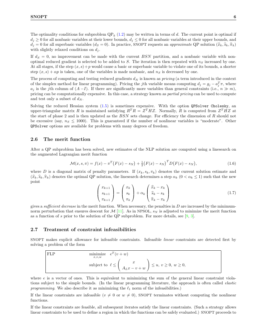
2.6
2.7
Introduction . . . . . . . . . . . . . . . . . . . . . . . . . . . . . . . . . . . . . . . . . .
Problem Types . . . . . . . . . . . . . . . . . . . . . . . . . . . . . . . . . . . . . . . . .
Selecting the SNOPT Solver . . . . . . . . . . . . . . . . . . . . . . . . . . . . . . . . . .
Description of the method . . . . . . . . . . . . . . . . . . . . . . . . . . . . . . . . . .
Objective function reconstruction . . . . . . . . . . . . . . . . . . . . . . . . . . . . . . .
Constraints and slack variables . . . . . . . . . . . . . . . . . . . . . . . . . . . . . . . .
. . . . . . . . . . . . . . . . . . . . . . . . . . . . . . . . . . . . . . . .
Major iterations
. . . . . . . . . . . . . . . . . . . . . . . . . . . . . . . . . . . . . . . .
Minor iterations
The reduced Hessian and reduced gradient
. . . . . . . . . . . . . . . . . . . . . . . . .
The merit function . . . . . . . . . . . . . . . . . . . . . . . . . . . . . . . . . . . . . . .
. . . . . . . . . . . . . . . . . . . . . . . . . . . .
Treatment of constraint infeasibilities
. . . . . . . . . . . . . . . . . . . . . . . . . . . .
Starting points . . . . . . . . . . . . . . . . . . . . . . . . . . . . . . . . . . . . . . . . .
Advanced basis . . . . . . . . . . . . . . . . . . . . . . . . . . . . . . . . . . . . . . . . .
. . . . . . . . . . . . . . . . . . . . . . . . . . . . . . . . . . . . . . . . . . . . .
GAMS options . . . . . . . . . . . . . . . . . . . . . . . . . . . . . . . . . . . . . . . . .
Model suffices . . . . . . . . . . . . . . . . . . . . . . . . . . . . . . . . . . . . . . . . . .
SNOPT options . . . . . . . . . . . . . . . . . . . . . . . . . . . . . . . . . . . . . . . . .
The SNOPT log . . . . . . . . . . . . . . . . . . . . . . . . . . . . . . . . . . . . . . . .
EXIT conditions . . . . . . . . . . . . . . . . . . . . . . . . . . . . . . . . . . . . . . . .
Listing file messages . . . . . . . . . . . . . . . . . . . . . . . . . . . . . . . . . . . . . .
Starting points and advanced bases
Options
3.1
3.2
4.1
4.2
4.3
5.1
1
2
2
2
3
3
4
4
5
6
6
7
7
8
9
9
11
12
22
27
30
1
Introduction
This section describes the GAMS interface to the general-purpose NLP solver SNOPT, (Sparse Nonlinear Opti-
mizer) which implements a sequential quadratic programming (SQP) method for solving constrained optimization
problems with smooth nonlinear functions in the objective and constraints. The optimization problem is assumed
to be stated in the form
NP
minimize
x
x
or maximize
f (x) ∼ b1
ALx ∼ b2
l ≤ x ≤ u,
subject to
f0(x)
(1.1)
�
SNOPT
2
where x ∈ n, f0(x) is a linear or nonlinear smooth objective function, l and u are constant lower and upper
bounds, f (x) is a set of nonlinear constraint functions, AL is a sparse matrix, ∼ is a vector of relational operators
(≤, ≥ or =), and b1 and b2 are right-hand side constants. f (x) ∼ b1 are the nonlinear constraints of the model
and ALx ∼ b2 form the linear constraints.
The gradients of f0 and fi are automatically provided by GAMS, using its automatic differentiation engine.
The bounds may include special values -INF or +INF to indicate lj = −∞ or uj = +∞ for appropriate j. Free
variables have both bounds infinite and fixed variables have lj = uj.
1.1 Problem Types
If the nonlinear functions are absent, the problem is a linear program (LP) and SNOPT applies the primal simplex
method [2]. Sparse basis factors are maintained by LUSOL [13] as in MINOS [16].
If only the objective is nonlinear, the problem is linearly constrained (LC) and tends to solve more easily than
the general case with nonlinear constraints (NC). Note that GAMS models have an objective variable instead of
an objective function. The GAMS/SNOPT link will try to substitute out the objective variable and reformulate
the model such that SNOPT will see a true objective function.
For both linearly and nonlinearly constrained problems SNOPT applies a sparse sequential quadratic programming
(SQP) method [6], using limited-memory quasi-Newton approximations to the Hessian of the Lagrangian. The
merit function for steplength control is an augmented Lagrangian, as in the dense SQP solver NPSOL [9, 11].
In general, SNOPT requires less matrix computation than NPSOL and fewer evaluations of the functions than the
nonlinear algorithms in MINOS [14, 15]. It is suitable for nonlinear problems with thousands of constraints and
variables, and is most efficient if only some of the variables enter nonlinearly, or there are relatively few degrees
of freedom at a solution (i.e., many constraints are active). However, unlike previous versions of SNOPT, there is
no limit on the number of degrees of freedom.
1.2 Selecting the SNOPT Solver
The GAMS system can be instructed to use the SNOPT solver by incorporating the following option in the GAMS
model:
option NLP=SNOPT;
If the model contains non-smooth functions like abs(x), or max(x, y) you can try to get it solved by SNOPT using
option DNLP=SNOPT;
These models have discontinuous derivatives however, and SNOPT was not designed for solving such models.
Discontinuities in the gradients can sometimes be tolerated if they are not too close to an optimum.
It is also possible to specify NLP=SNOPT or DNLP=SNOPT on the command line, as in:
> gamslib chem
> gams chem nlp=snopt
In the Windows IDE command line parameters can be specified in the parameter combo box above the edit
window.
2 Description of the method
Here we briefly describe the main features of the SQP algorithm used in SNOPT and introduce some terminology.
The SQP algorithm is fully described by by Gill, Murray and Saunders[7].
�
SNOPT
3
2.1 Objective function reconstruction
The first step GAMS/SNOPT performs is to try to reconstruct the objective function. In GAMS, optimization
models minimize or maximize an objective variable. SNOPT however works with an objective function. One way
of dealing with this is to add a dummy linear function with just the objective variable. Consider the following
GAMS fragment:
obj.. z =e= sum(i, sqr[r(i)]);
model m /all/;
solve m using nlp minimizing z;
This can be cast in form (1.1) by saying minimize z subject to z =
to minimize the nonlinear expression
i and the other constraints in the model.
Although simple, this approach is not always preferable. Especially when all constraints are linear it is important
i directly. This can be achieved by a simple reformulation: z can be
substituted out. The substitution mechanism carries out the formulation if all of the following conditions hold:
i r2
i r2
• the objective variable z is a free continuous variable (no bounds are defined on z),
• z appears linearly in the objective function,
• the objective function is formulated as an equality constraint,
• z is only present in the objective function and not in other constraints.
For many models it is very important that the nonlinear objective function be used by SNOPT. For instance the
model chem.gms from the model library solves in 16 iterations. When we add the bound
energy.lo = 0;
on the objective variable energy and thus preventing it from being substituted out, SNOPT will not be able to
find a feasible point for the given starting point.
This reformulation mechanism has been extended for substitutions along the diagonal. For example, the GAMS
model
variables x,y,z;
equations e1,e2;
e1..z =e= y;
e2..y =e= sqr(1+x);
model m /all/;
option nlp=snopt;
solve m using nlp minimizing z;
will be reformulated as an unconstrained optimization problem
minimize f (x) = (1 + x)2.
These additional reformulations can be turned off by using the statement option reform = 0; (see §4.1).
2.2 Constraints and slack variables
Problem (1.1) contains n variables in x. Let m be the number of components of f (x) and ALx combined. The
upper and lower bounds on those terms define the general constraints of the problem. SNOPT converts the
general constraints to equalities by introducing a set of slack variables s = (s1, s2, ..., sm)T . For example, the
linear constraint 5 ≤ 2x1 + 3x2 ≤ +∞ is replaced by 2x1 + 3x2 − s1 = 0 together with the bounded slack
5 ≤ s1 ≤ +∞. Problem (1.1) can be written in the equivalent form
�
SNOPT
4
minimize
x,s
subject to
f0(x)
f (x)
ALx
x
s
≤ u.
− s = 0,
l ≤
where a maximization problem is cast into a minimization by multiplying the objective function by −1.
The linear and nonlinear general constraints become equalities of the form f (x) − sN = 0 and ALx − sL = 0,
where sL and sN are known as the linear and nonlinear slacks.
2.3 Major iterations
The basic structure of SNOPT’s solution algorithm involves major and minor iterations. The major iterations
generate a sequence of iterates (xk) that satisfy the linear constraints and converge to a point that satisfies the
first-order conditions for optimality. At each iterate {xk} a QP subproblem is used to generate a search direction
towards the next iterate {xk+1}. The constraints of the subproblem are formed from the linear constraints
ALx − sL = 0 and the nonlinear constraint linearization
f (xk) + f(xk)(x − xk) − sN = 0,
where f(xk) denotes the Jacobian: a matrix whose rows are the first derivatives of f (x) evaluated at xk. The
QP constraints therefore comprise the m linear constraints
f(xk)x −sN
ALx
= −f (xk) + f(xk)xk,
−sL = 0,
where x and s are bounded by l and u as before. If the m × n matrix A and m-vector b are defined as
−f (xk) + f(xk)xk
,
0
f(xk)
AL
A =
and b =
then the QP subproblem can be written as
QPk
x,s
minimize
q(x, xk) = gT
subject to Ax − s = b,
k (x − xk) +
l ≤
x
s
(x − xk)T Hk(x − xk)
1
2
≤ u,
(1.2)
where q(x, xk) is a quadratic approximation to a modified Lagrangian function [6]. The matrix Hk is a quasi-
Newton approximation to the Hessian of the Lagrangian. A BFGS update is applied after each major iteration.
If some of the variables enter the Lagrangian linearly the Hessian will have some zero rows and columns. If the
nonlinear variables appear first, then only the leading n1 rows and columns of the Hessian need be approximated,
where n1 is the number of nonlinear variables.
2.4 Minor iterations
Solving the QP subproblem is itself an iterative procedure. Here, the iterations of the QP solver SQOPT[8] form
the minor iterations of the SQP method.
SQOPT uses a reduced-Hessian active-set method implemented as a reduced-gradient method similar to that in
MINOS [14].
At each minor iteration, the constraints Ax − s = b are partitioned into the form
BxB + SxS + N xN = b,
�
SNOPT
5
where the basis matrix B is square and nonsingular and the matrices S, N are the remaining columns of (A −I).
The vectors xB, xS, xN are the associated basic, superbasic, and nonbasic variables components of (x, s).
The term active-set method arises because the nonbasic variables xN are temporarily frozen at their upper or
lower bounds, and their bounds are considered to be active. Since the general constraints are satisfied also, the
set of active constraints takes the form
xB
xS
xN
=
,
b
xN
B S N
I
where xN represents the current values of the nonbasic variables. (In practice, nonbasic variables are sometimes
frozen at values strictly between their bounds.) The reduced-gradient method chooses to move the superbasic
variables in a direction that will improve the objective function. The basic variables “tag along” to keep Ax−s = b
satisfied, and the nonbasic variables remain unaltered until one of them is chosen to become superbasic.
At a nonoptimal feasible point (x, s) we seek a search direction p such that (x, s) + p remains on the set of active
constraints yet improves the QP objective. If the new point is to be feasible, we must have BpB + SpS + N pN = 0
and pN = 0. Once pS is specified, pB is uniquely determined from the system BpB = −SpS. It follows that the
superbasic variables may be regarded as independent variables that are free to move in any desired direction. The
number of superbasic variables (nS say) therefore indicates the number of degrees of freedom remaining after the
constraints have been satisfied. In broad terms, nS is a measure of how nonlinear the problem is. In particular,
nS need not be more than one for linear problems.
2.5 The reduced Hessian and reduced gradient
The dependence of p on pS may be expressed compactly as p = ZpS, where Z is a matrix that spans the null
space of the active constraints:
−B−1S
I
0
Z = P
(1.3)
where P permutes the columns of (A −I) into the order (B S N ). Minimizing q(x, xk) with respect to pS now
involves a quadratic function of pS:
gT ZpS +
pT
S Z T HZpS,
(1.4)
1
2
where g and H are expanded forms of gk and Hk defined for all variables (x, s). This is a quadratic with
Hessian Z T HZ (the reduced Hessian) and constant vector Z T g (the reduced gradient). If the reduced Hessian is
nonsingular, pS is computed from the system
Z T HZpS = −Z T g.
(1.5)
The matrix Z is used only as an operator, i.e., it is not stored explicitly. Products of the form Zv or Z T g are
obtained by solving with B or BT . The package LUSOL[13] is used to maintain sparse LU factors of B as the
BSN partition changes. From the definition of Z, we see that the reduced gradient can be computed from
BT π = gB, Z T g = gS − ST π,
where π is an estimate of the dual variables associated with the m equality constraints Ax − s = b, and gB is the
basic part of g.
By analogy with the elements of Z T g, we define a vector of reduced gradients (or reduced costs) for all variables
in (x, s):
d = g −
AT
−I
π,
so that dS = Z T g.
At a feasible point, the reduced gradients for the slacks s are the dual variables π.
�
SNOPT
6
The optimality conditions for subproblem QPk (1.2) may be written in terms of d. The current point is optimal if
dj ≥ 0 for all nonbasic variables at their lower bounds, dj ≤ 0 for all nonbasic variables at their upper bounds, and
dj = 0 for all superbasic variables (dS = 0). In practice, SNOPT requests an approximate QP solution (xk,sk,πk)
with slightly relaxed conditions on dj.
If dS = 0, no improvement can be made with the current BSN partition, and a nonbasic variable with non-
optimal reduced gradient is selected to be added to S. The iteration is then repeated with nS increased by one.
At all stages, if the step (x, s) + p would cause a basic or superbasic variable to violate one of its bounds, a shorter
step (x, s) + αp is taken, one of the variables is made nonbasic, and nS is decreased by one.
The process of computing and testing reduced gradients dN is known as pricing (a term introduced in the context
of the simplex method for linear programming). Pricing the jth variable means computing dj = gj − aT
j π, where
aj is the jth column of (A −I). If there are significantly more variables than general constraints (i.e., n m),
pricing can be computationally expensive. In this case, a strategy known as partial pricing can be used to compute
and test only a subset of dN .
Solving the reduced Hessian system (1.5) is sometimes expensive. With the option QPSolver Cholesky, an
upper-triangular matrix R is maintained satisfying RT R = Z T HZ. Normally, R is computed from Z T HZ at
the start of phase 2 and is then updated as the BSN sets change. For efficiency the dimension of R should not
be excessive (say, nS ≤ 1000). This is guaranteed if the number of nonlinear variables is “moderate”. Other
QPSolver options are available for problems with many degrees of freedom.
2.6 The merit function
After a QP subproblem has been solved, new estimates of the NLP solution are computed using a linesearch on
the augmented Lagrangian merit function
where D is a diagonal matrix of penalty parameters. If (xk, sk, πk) denotes the current solution estimate and
(xk,sk,πk) denotes the optimal QP solution, the linesearch determines a step αk (0 < αk ≤ 1) such that the new
2
point
DF (x) − sN
T
F (x) − sN
+ 1
M(x, s, π) = f (x) − πTF (x) − sN
xk
xk − xk
+ αk
sk − sk
πk − πk
xk+1
=
sk+1
πk+1
sk
πk
,
(1.6)
(1.7)
gives a sufficient decrease in the merit function. When necessary, the penalties in D are increased by the minimum-
norm perturbation that ensures descent for M [11]. As in NPSOL, sN is adjusted to minimize the merit function
as a function of s prior to the solution of the QP subproblem. For more details, see [9, 3].
2.7 Treatment of constraint infeasibilities
SNOPT makes explicit allowance for infeasible constraints.
solving a problem of the form
Infeasible linear constraints are detected first by
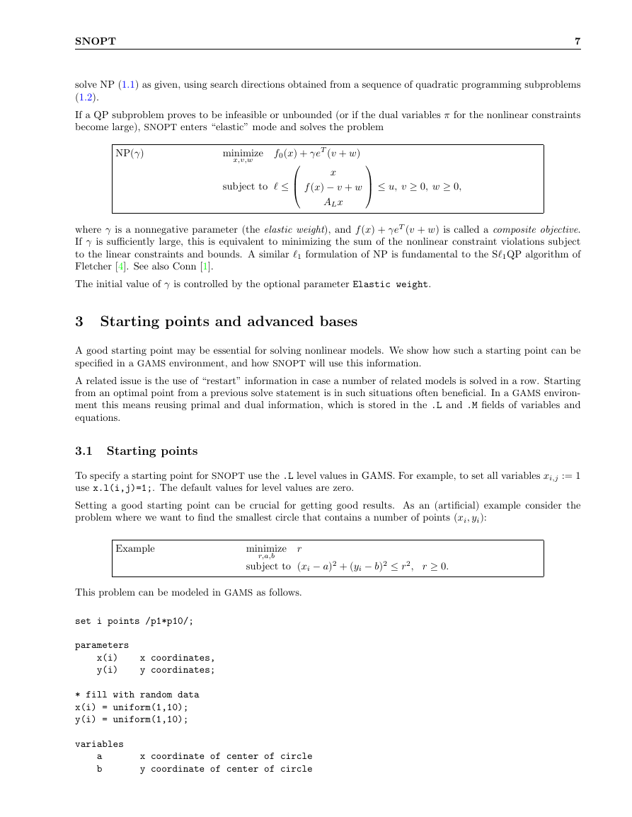
FLP
minimize
x,v,w
eT (v + w)
≤ u, v ≥ 0, w ≥ 0,
subject to ≤
x
ALx − v + w
where e is a vector of ones. This is equivalent to minimizing the sum of the general linear constraint viola-
tions subject to the simple bounds. (In the linear programming literature, the approach is often called elastic
programming. We also describe it as minimizing the 1 norm of the infeasibilities.)
If the linear constraints are infeasible (v = 0 or w = 0), SNOPT terminates without computing the nonlinear
functions.
If the linear constraints are feasible, all subsequent iterates satisfy the linear constraints. (Such a strategy allows
linear constraints to be used to define a region in which the functions can be safely evaluated.) SNOPT proceeds to
�
SNOPT
7
solve NP (1.1) as given, using search directions obtained from a sequence of quadratic programming subproblems
(1.2).
If a QP subproblem proves to be infeasible or unbounded (or if the dual variables π for the nonlinear constraints
become large), SNOPT enters “elastic” mode and solves the problem
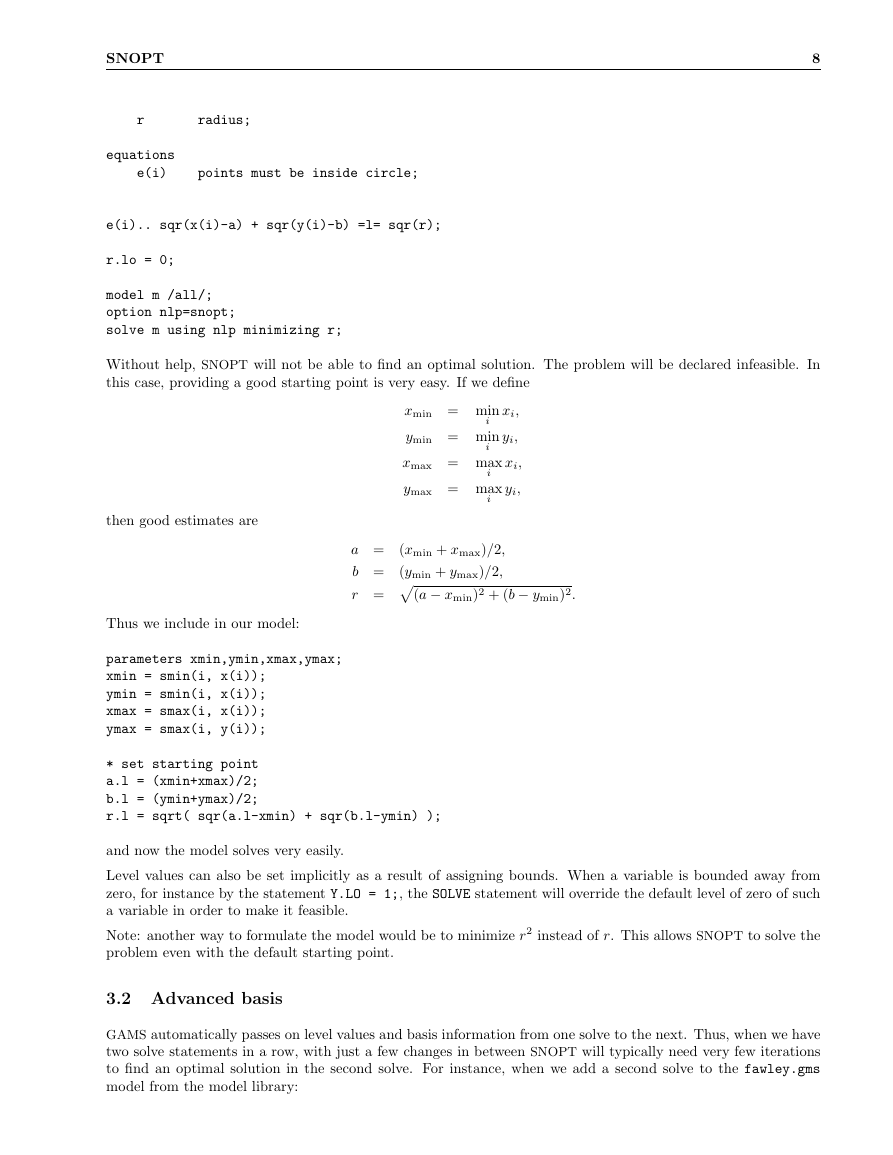
NP(γ)
minimize
x,v,w
f0(x) + γeT (v + w)
subject to ≤
x
f (x) − v + w
ALx
≤ u, v ≥ 0, w ≥ 0,
where γ is a nonnegative parameter (the elastic weight), and f (x) + γeT (v + w) is called a composite objective.
If γ is sufficiently large, this is equivalent to minimizing the sum of the nonlinear constraint violations subject
to the linear constraints and bounds. A similar 1 formulation of NP is fundamental to the S1QP algorithm of
Fletcher [4]. See also Conn [1].
The initial value of γ is controlled by the optional parameter Elastic weight.
3 Starting points and advanced bases
A good starting point may be essential for solving nonlinear models. We show how such a starting point can be
specified in a GAMS environment, and how SNOPT will use this information.
A related issue is the use of “restart” information in case a number of related models is solved in a row. Starting
from an optimal point from a previous solve statement is in such situations often beneficial. In a GAMS environ-
ment this means reusing primal and dual information, which is stored in the .L and .M fields of variables and
equations.
3.1 Starting points
To specify a starting point for SNOPT use the .L level values in GAMS. For example, to set all variables xi,j := 1
use x.l(i,j)=1;. The default values for level values are zero.
Setting a good starting point can be crucial for getting good results. As an (artificial) example consider the
problem where we want to find the smallest circle that contains a number of points (xi, yi):
Example
r
minimize
subject to (xi − a)2 + (yi − b)2 ≤ r2, r ≥ 0.
r,a,b
This problem can be modeled in GAMS as follows.
set i points /p1*p10/;
parameters
x(i)
y(i)
x coordinates,
y coordinates;
* fill with random data
x(i) = uniform(1,10);
y(i) = uniform(1,10);
variables
a
b
x coordinate of center of circle
y coordinate of center of circle
�
8
SNOPT
r
radius;
equations
e(i)
points must be inside circle;
e(i).. sqr(x(i)-a) + sqr(y(i)-b) =l= sqr(r);
r.lo = 0;
model m /all/;
option nlp=snopt;
solve m using nlp minimizing r;
Without help, SNOPT will not be able to find an optimal solution. The problem will be declared infeasible. In
this case, providing a good starting point is very easy. If we define
then good estimates are
xmin = min
i
ymin = min
i
xi,
yi,
xmax = max
i
ymax = max
i
xi,
yi,
a = (xmin + xmax)/2,
b = (ymin + ymax)/2,
r = (a − xmin)2 + (b − ymin)2.
Thus we include in our model:
parameters xmin,ymin,xmax,ymax;
xmin = smin(i, x(i));
ymin = smin(i, x(i));
xmax = smax(i, x(i));
ymax = smax(i, y(i));
* set starting point
a.l = (xmin+xmax)/2;
b.l = (ymin+ymax)/2;
r.l = sqrt( sqr(a.l-xmin) + sqr(b.l-ymin) );
and now the model solves very easily.
Level values can also be set implicitly as a result of assigning bounds. When a variable is bounded away from
zero, for instance by the statement Y.LO = 1;, the SOLVE statement will override the default level of zero of such
a variable in order to make it feasible.
Note: another way to formulate the model would be to minimize r2 instead of r. This allows SNOPT to solve the
problem even with the default starting point.
3.2 Advanced basis
GAMS automatically passes on level values and basis information from one solve to the next. Thus, when we have
two solve statements in a row, with just a few changes in between SNOPT will typically need very few iterations
to find an optimal solution in the second solve. For instance, when we add a second solve to the fawley.gms
model from the model library:
�



 2023年江西萍乡中考道德与法治真题及答案.doc
 2012年重庆南川中考生物真题及答案.doc
 2013年江西师范大学地理学综合及文艺理论基础考研真题.doc
 2020年四川甘孜小升初语文真题及答案I卷.doc
 2020年注册岩土工程师专业基础考试真题及答案.doc
 2023-2024学年福建省厦门市九年级上学期数学月考试题及答案.doc
 2021-2022学年辽宁省沈阳市大东区九年级上学期语文期末试题及答案.doc
 2022-2023学年北京东城区初三第一学期物理期末试卷及答案.doc
 2018上半年江西教师资格初中地理学科知识与教学能力真题及答案.doc
 2012年河北国家公务员申论考试真题及答案-省级.doc
 2020-2021学年江苏省扬州市江都区邵樊片九年级上学期数学第一次质量检测试题及答案.doc
 2022下半年黑龙江教师资格证中学综合素质真题及答案.doc