点云分割基于特征边界提取.pdf

发布时间：2022-06-02 发布人：admin 分类：说明书资料大小：0.94M 资料格式：pdf 举报版权申诉

第1页 / 共8页

第2页 / 共8页

第3页 / 共8页

第4页 / 共8页

第5页 / 共8页

第6页 / 共8页

第7页 / 共8页

第8页 / 共8页

Detection of closed sharp edges in point clouds using normal estimation and graph theory

Introduction

Sharp feature line extraction algorithm

Algorithm overview

First order segmentation of point cloud

Building graph Gall of all clusters

Adding edges to the graph Gall yielding Gextended

Building Gpruned_mst , the pruned minimum spanning tree of Gextended

Construction of Gpruned_branches by pruning short branches in Gpruned_mst

Building Gclosed by closing the sharp feature lines in Gpruned_branches

Generating Gsmooth by smoothing Gclosed

Results

Conclusion and future work

Acknowledgement

References

Computer-Aided Design 39 (2007) 276–283 www.elsevier.com/locate/cad Detection of closed sharp edges in point clouds using normal estimation and graph theory Kris Demarsina,∗, Denis Vanderstraetenb, Tim Volodinea, Dirk Roosea a Katholieke Universiteit Leuven, Department of Computer Science, Celestijnenlaan 200A, 3001 Heverlee, Belgium b Metris N.V., Interleuvenlaan 86, B-3001 Leuven, Belgium Received 18 May 2006; accepted 17 December 2006 Abstract The reconstruction of a surface model from a point cloud is an important task in the reverse engineering of industrial parts. We aim at constructing a curve network on the point cloud that will deﬁne the border of the various surface patches. In this paper, we present an algorithm to extract closed sharp feature lines, which is necessary to create such a closed curve network. We use a ﬁrst order segmentation to extract candidate feature points and process them as a graph to recover the sharp feature lines. To this end, a minimum spanning tree is constructed and afterwards a reconnection procedure closes the lines. The algorithm is fast and gives good results for real-world point sets from industrial applications. c 2007 Elsevier Ltd. All rights reserved. Keywords: Reverse engineering; Segmentation; Region growing; Sharp edges; Point clouds; Curve network 1. Introduction Feature lines on a surface model can be mathematically deﬁned via local extrema of principal curvatures along corresponding principal directions. These feature lines can be used in a variety of applications, e.g. visualization, improvement of the mesh quality, shape recognition, quality control and reverse engineering. Most feature line extraction algorithms rely on a triangular mesh as input, e.g. [1–5]. Few algorithms only use a point cloud, e.g. [6,7]. These existing methods usually result in pieces of unconnected feature lines, making it hard to segment a point cloud or mesh into surface patches, based on these lines. A method to ﬁnd the different surface patches with corresponding boundaries is presented in [8]. This method relies on a triangular mesh as input, but sometimes a mesh is not given or it can be hard to generate one. A segmentation algorithm that operates on point clouds is explained in [9]. This method uses curvature information that is difﬁcult to estimate in a noisy environment. In this paper, we aim at constructing a curve network on a point cloud that will deﬁne the border of the various surface ∗ Corresponding author. E-mail address: kris.demarsin@cs.kuleuven.be (K. Demarsin). 0010-4485/$ - see front matter c 2007 Elsevier Ltd. All rights reserved. doi:10.1016/j.cad.2006.12.005 patches. Therefore, we focus on ﬁnding closed sharp feature lines. Our method can be sketched as follows. First, a region growing method is applied with normal estimation, which is a modiﬁcation of the method of Vanco et al. [10–12], to cluster the points in order to reduce the point cloud size. We build and manipulate a graph of these clusters, resulting in closed sharp feature lines that ﬁt the clusters such that the algorithm can be used as a pre-process step to ﬁnd the areas where a surface patch can be deﬁned. We are interested in point clouds from industrial applications, where closed sharp feature lines can be detected. It is not our goal to apply the algorithm to point clouds with free form surfaces or ﬁllets with a large radius. The algorithm differs from existing feature line algorithms by the fact that it reconstructs closed sharp feature lines. The advantages of the algorithm are that (a) it is meshless, i.e. only the coordinates of the points are used, (b) it intelligently clusters the points to create a graph that is much smaller than the original cloud, thus making it practical for large point clouds and, (c) it constitutes a pre-process step for surface reconstruction. An introduction to the algorithm, together with some results, is published in [13]. In this paper, the algorithm is explained in detail (see Section 2). In Section 3 we illustrate results of the algorithm applied to realistic point clouds, i.e. point

K. Demarsin et al. / Computer-Aided Design 39 (2007) 276–283 277 Algorithm 1 High level description of the algorithm. 1. Segment point cloud using the normals ⇒ point clusters (clusters) (Fig. 1) 2. Build graph Gall connecting neighboring clusters (Figs. 2 and 3(a)) 3. Add edges, indicating a piece of a sharp feature line, to Gall ⇒ Gextended (Fig. 3(b)) 4. Build the pruned minimum spanning tree of Gextended ⇒ Gpruned mst (Fig. 3(c)) 5. Prune short branches in Gpruned mst ⇒ Gpruned branches (Fig. 3(d)) 6. Close the sharp feature lines in Gpruned branches ⇒ Gclosed (Fig. 3(e)) 7. Smooth the sharp feature lines in Gclosed ⇒ Gsmooth (Fig. 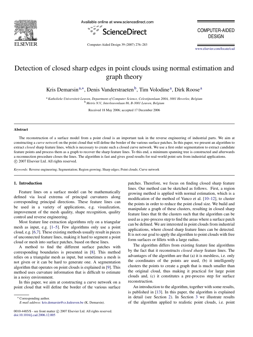3(f)) Fig. 1. First order segmentation of two intersecting cylinders. one side, which is undesirable in our algorithm. If a triangular mesh is available, the 1-ring neighborhood of p can be used to represent a good local neighborhood of p, with the neighbors distributed around p. In the absence of a mesh, we approximate this neighborhood by building a local mesh. We determine the k nearest neighbors of p, with k large enough, by generating a sphere with p as midpoint and a radius such that the k nearest neighbors are inside this sphere. Then the least squares plane through these points is constructed and the points are projected on this plane. Next, we compute the Delaunay triangulation of these projected points and only the points that share an edge with p in this triangulation, constitute the Delaunay neighborhood [14] of p, which is used as an approximation of the 1-ring neighborhood. The normal in p is estimated as the normal of the least squares plane through the 1-ring neighborhood of p, as explained in [15]. Since we only use a few points from the k nearest neighbors (the 1-ring neighborhood), the value of k has not much inﬂuence on the normal estimation when k is chosen large enough. Consequently, setting the value of this parameter to 20 was suitable for all the tested point clouds. Region growing. We want to use a standard region growing method to cluster the points based on the sharp edges using only normal estimation. Hence, we use a modiﬁcation of the ﬁrst order segmentation described by Vanco et al. [10–12]: only one threshold angle αmax is used which speciﬁes the maximum acceptable angle between the normals of two adjacent points in one cluster. At a sharp edge, the normal estimation depends heavily on the computed 1-ring neighborhood, since this neighborhood is very local and these neighbors are located on both sides of the sharp edge. This means that the variation of the normals along a sharp edge is high, resulting in large clusters with low variation of the normals bounded by small clusters with high normal variation. These small clusters indicate the sharp edges. Fig. 1 illustrates the result of the ﬁrst order segmentation, applied to the point cloud of the two intersecting cylinders, with each point colored corresponding to the cluster it belongs to. Contrary to the method of Vanco et al. [10–12], each cylindrical piece, bounded by sharp edges, consists of only one large cluster with many small clusters deﬁning the boundary. 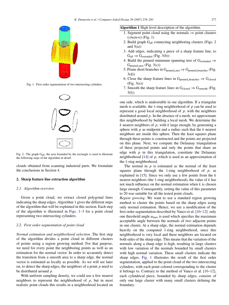Fig. 2. The graph Gall; the area bounded by the rectangle is used to illustrate the following steps of the algorithm in detail. clouds obtained from scanning industrial parts. We formulate the conclusions in Section 4. 2. Sharp feature line extraction algorithm 2.1. Algorithm overview Given a point cloud, we extract closed polygonal lines indicating the sharp edges. Algorithm 1 gives the different steps of the algorithm that will be explained in this section. Each step of the algorithm is illustrated in Figs. 1–3 for a point cloud representing two intersecting cylinders. 2.2. First order segmentation of point cloud Normal estimation and neighborhood selection. The ﬁrst step of the algorithm divides a point cloud in different clusters of points using a region growing method. For that purpose, we need for every point the neighboring points as well as an estimation for the normal vector. In order to accurately detect the transition from a smooth area to a sharp edge, the normal vector is estimated as locally as possible. As we will see later on, to detect the sharp edges, the neighbors of a point p need to be distributed around p. With uniform sampling density, we could use a few nearest neighbors to represent the neighborhood of p, but in most realistic point clouds this results in a neighborhood located on

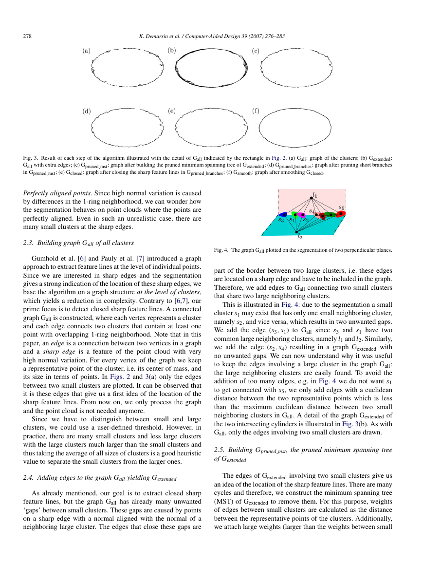
278 K. Demarsin et al. / Computer-Aided Design 39 (2007) 276–283 Fig. 3. Result of each step of the algorithm illustrated with the detail of Gall indicated by the rectangle in Fig. 2. (a) Gall: graph of the clusters; (b) Gextended: Gall with extra edges; (c) Gpruned mst: graph after building the pruned minimum spanning tree of Gextended; (d) Gpruned branches: graph after pruning short branches in Gpruned mst; (e) Gclosed: graph after closing the sharp feature lines in Gpruned branches; (f) Gsmooth: graph after smoothing Gclosed. Perfectly aligned points. Since high normal variation is caused by differences in the 1-ring neighborhood, we can wonder how the segmentation behaves on point clouds where the points are perfectly aligned. Even in such an unrealistic case, there are many small clusters at the sharp edges. 2.3. Building graph Gall of all clusters Gumhold et al. [6] and Pauly et al. [7] introduced a graph approach to extract feature lines at the level of individual points. Since we are interested in sharp edges and the segmentation gives a strong indication of the location of these sharp edges, we base the algorithm on a graph structure at the level of clusters, which yields a reduction in complexity. Contrary to [6,7], our prime focus is to detect closed sharp feature lines. A connected graph Gall is constructed, where each vertex represents a cluster and each edge connects two clusters that contain at least one point with overlapping 1-ring neighborhood. Note that in this paper, an edge is a connection between two vertices in a graph and a sharp edge is a feature of the point cloud with very high normal variation. For every vertex of the graph we keep a representative point of the cluster, i.e. its center of mass, and its size in terms of points. In Figs. 2 and 3(a) only the edges between two small clusters are plotted. It can be observed that it is these edges that give us a ﬁrst idea of the location of the sharp feature lines. From now on, we only process the graph and the point cloud is not needed anymore. Since we have to distinguish between small and large clusters, we could use a user-deﬁned threshold. However, in practice, there are many small clusters and less large clusters with the large clusters much larger than the small clusters and thus taking the average of all sizes of clusters is a good heuristic value to separate the small clusters from the larger ones. 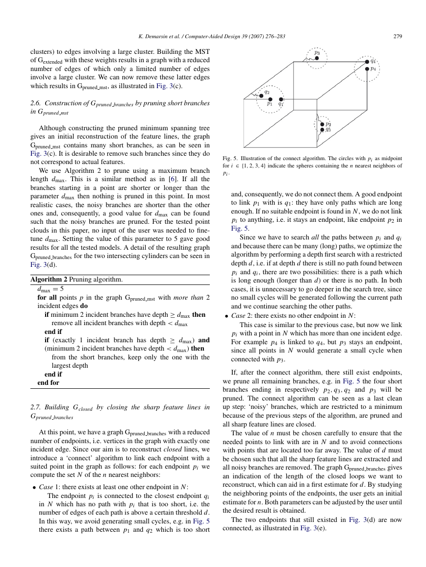Fig. 4. The graph Gall plotted on the segmentation of two perpendicular planes. part of the border between two large clusters, i.e. these edges are located on a sharp edge and have to be included in the graph. Therefore, we add edges to Gall connecting two small clusters that share two large neighboring clusters. This is illustrated in Fig. 4: due to the segmentation a small cluster s1 may exist that has only one small neighboring cluster, namely s2, and vice versa, which results in two unwanted gaps. We add the edge (s3, s1) to Gall since s3 and s1 have two common large neighboring clusters, namely l1 and l2. Similarly, we add the edge (s2, s4) resulting in a graph Gextended with no unwanted gaps. We can now understand why it was useful to keep the edges involving a large cluster in the graph Gall: the large neighboring clusters are easily found. To avoid the addition of too many edges, e.g. in Fig. 4 we do not want s1 to get connected with s5, we only add edges with a euclidean distance between the two representative points which is less than the maximum euclidean distance between two small neighboring clusters in Gall. A detail of the graph Gextended of the two intersecting cylinders is illustrated in Fig. 3(b). As with Gall, only the edges involving two small clusters are drawn. 2.5. Building Gpruned mst, the pruned minimum spanning tree of Gextended 2.4. Adding edges to the graph Gall yielding Gextended As already mentioned, our goal is to extract closed sharp feature lines, but the graph Gall has already many unwanted ‘gaps’ between small clusters. These gaps are caused by points on a sharp edge with a normal aligned with the normal of a neighboring large cluster. The edges that close these gaps are The edges of Gextended involving two small clusters give us an idea of the location of the sharp feature lines. There are many cycles and therefore, we construct the minimum spanning tree (MST) of Gextended to remove them. For this purpose, weights of edges between small clusters are calculated as the distance between the representative points of the clusters. Additionally, we attach large weights (larger than the weights between small

K. Demarsin et al. / Computer-Aided Design 39 (2007) 276–283 279 clusters) to edges involving a large cluster. Building the MST of Gextended with these weights results in a graph with a reduced number of edges of which only a limited number of edges involve a large cluster. We can now remove these latter edges which results in Gpruned mst, as illustrated in Fig. 3(c). 2.6. Construction of Gpruned branches by pruning short branches in Gpruned mst Although constructing the pruned minimum spanning tree gives an initial reconstruction of the feature lines, the graph Gpruned mst contains many short branches, as can be seen in Fig. 3(c). It is desirable to remove such branches since they do not correspond to actual features. We use Algorithm 2 to prune using a maximum branch length dmax. This is a similar method as in [6]. If all the branches starting in a point are shorter or longer than the parameter dmax then nothing is pruned in this point. In most realistic cases, the noisy branches are shorter than the other ones and, consequently, a good value for dmax can be found such that the noisy branches are pruned. For the tested point clouds in this paper, no input of the user was needed to ﬁne- tune dmax. Setting the value of this parameter to 5 gave good results for all the tested models. A detail of the resulting graph Gpruned branches for the two intersecting cylinders can be seen in Fig. 3(d). Algorithm 2 Pruning algorithm. dmax = 5 for all points p in the graph Gpruned mst with more than 2 incident edges do if minimum 2 incident branches have depth ≥ dmax then remove all incident branches with depth < dmax end if if (exactly 1 incident branch has depth ≥ dmax) and (minimum 2 incident branches have depth < dmax) then from the short branches, keep only the one with the largest depth end if end for 2.7. Building Gclosed by closing the sharp feature lines in Gpruned branches At this point, we have a graph Gpruned branches with a reduced number of endpoints, i.e. vertices in the graph with exactly one incident edge. Since our aim is to reconstruct closed lines, we introduce a ‘connect’ algorithm to link each endpoint with a suited point in the graph as follows: for each endpoint pi we compute the set N of the n nearest neighbors: • Case 1: there exists at least one other endpoint in N: The endpoint pi is connected to the closest endpoint qi in N which has no path with pi that is too short, i.e. the number of edges of each path is above a certain threshold d. In this way, we avoid generating small cycles, e.g. in Fig. 5 there exists a path between p1 and q2 which is too short Fig. 5. Illustration of the connect algorithm. The circles with pi as midpoint for i ∈ {1, 2, 3, 4} indicate the spheres containing the n nearest neighbors of pi . and, consequently, we do not connect them. A good endpoint to link p1 with is q1: they have only paths which are long enough. If no suitable endpoint is found in N, we do not link pi to anything, i.e. it stays an endpoint, like endpoint p2 in Fig. 5. Since we have to search all the paths between pi and qi and because there can be many (long) paths, we optimize the algorithm by performing a depth ﬁrst search with a restricted depth d, i.e. if at depth d there is still no path found between pi and qi , there are two possibilities: there is a path which is long enough (longer than d) or there is no path. In both cases, it is unnecessary to go deeper in the search tree, since no small cycles will be generated following the current path and we continue searching the other paths. • Case 2: there exists no other endpoint in N: This case is similar to the previous case, but now we link pi with a point in N which has more than one incident edge. For example p4 is linked to q4, but p3 stays an endpoint, since all points in N would generate a small cycle when connected with p3. If, after the connect algorithm, there still exist endpoints, we prune all remaining branches, e.g. in Fig. 5 the four short branches ending in respectively p2, q3, q2 and p3 will be pruned. The connect algorithm can be seen as a last clean up step: ‘noisy’ branches, which are restricted to a minimum because of the previous steps of the algorithm, are pruned and all sharp feature lines are closed. The value of n must be chosen carefully to ensure that the needed points to link with are in N and to avoid connections with points that are located too far away. The value of d must be chosen such that all the sharp feature lines are extracted and all noisy branches are removed. The graph Gpruned branches gives an indication of the length of the closed loops we want to reconstruct, which can aid in a ﬁrst estimate for d. By studying the neighboring points of the endpoints, the user gets an initial estimate for n. Both parameters can be adjusted by the user until the desired result is obtained. The two endpoints that still existed in Fig. 3(d) are now connected, as illustrated in Fig. 3(e).

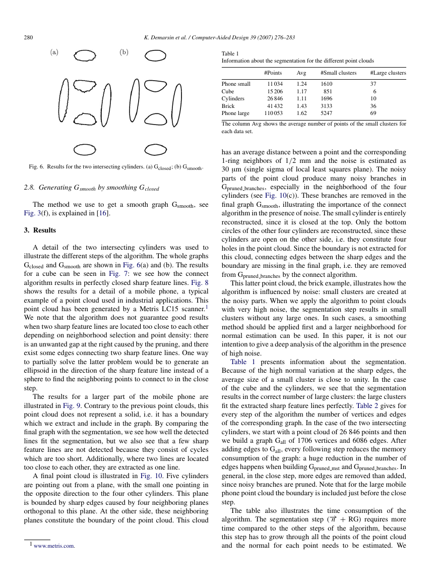
280 K. Demarsin et al. / Computer-Aided Design 39 (2007) 276–283 Table 1 Information about the segmentation for the different point clouds #Points Avg #Small clusters #Large clusters 11 034 15 206 26 846 41 432 110 053 Phone small Cube Cylinders Brick Phone large The column Avg shows the average number of points of the small clusters for each data set. 1610 851 1696 3133 5247 1.24 1.17 1.11 1.43 1.62 37 6 10 36 69 Fig. 6. Results for the two intersecting cylinders. (a) Gclosed; (b) Gsmooth. 2.8. Generating Gsmooth by smoothing Gclosed The method we use to get a smooth graph Gsmooth, see Fig. 3(f), is explained in [16]. 3. Results A detail of the two intersecting cylinders was used to illustrate the different steps of the algorithm. The whole graphs Gclosed and Gsmooth are shown in Fig. 6(a) and (b). 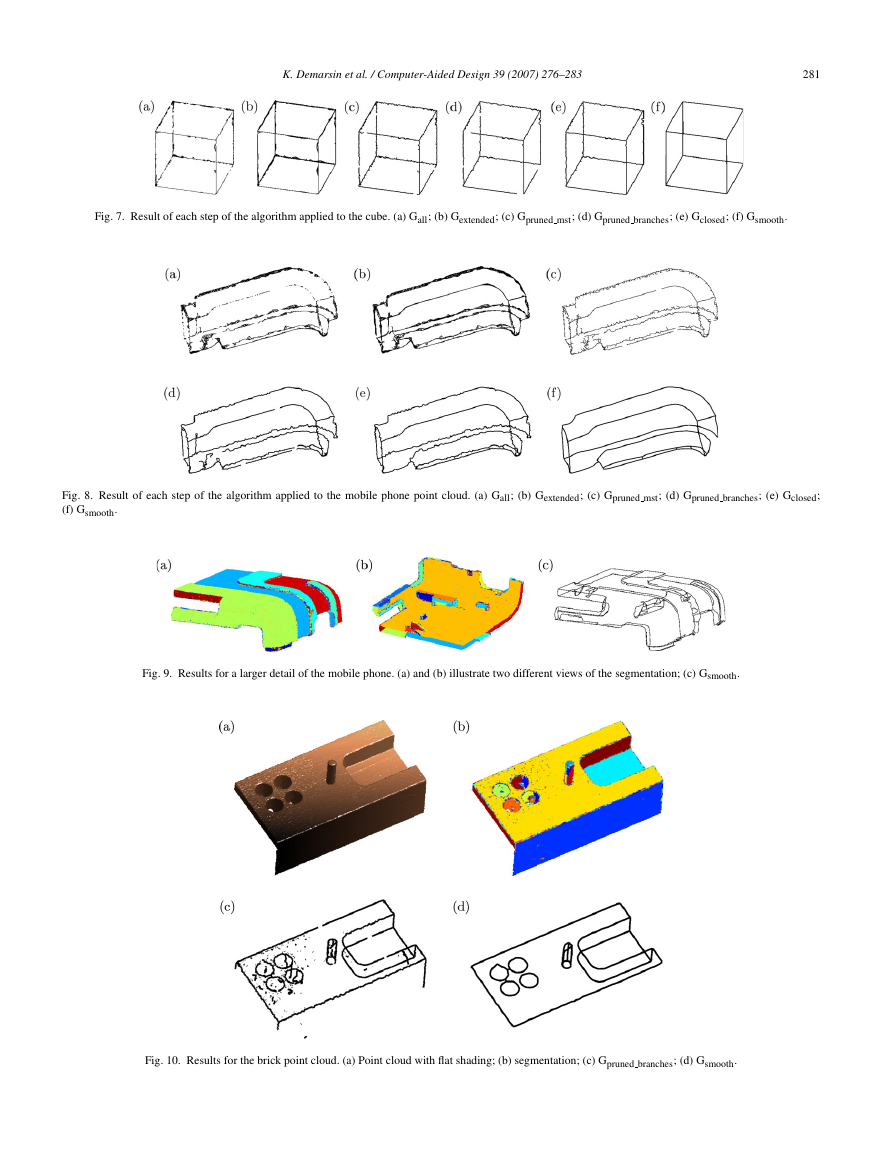The results for a cube can be seen in Fig. 7: we see how the connect algorithm results in perfectly closed sharp feature lines. Fig. 8 shows the results for a detail of a mobile phone, a typical example of a point cloud used in industrial applications. This point cloud has been generated by a Metris LC15 scanner.1 We note that the algorithm does not guarantee good results when two sharp feature lines are located too close to each other depending on neighborhood selection and point density: there is an unwanted gap at the right caused by the pruning, and there exist some edges connecting two sharp feature lines. One way to partially solve the latter problem would be to generate an ellipsoid in the direction of the sharp feature line instead of a sphere to ﬁnd the neighboring points to connect to in the close step. The results for a larger part of the mobile phone are illustrated in Fig. 9. Contrary to the previous point clouds, this point cloud does not represent a solid, i.e. it has a boundary which we extract and include in the graph. By comparing the ﬁnal graph with the segmentation, we see how well the detected lines ﬁt the segmentation, but we also see that a few sharp feature lines are not detected because they consist of cycles which are too short. Additionally, where two lines are located too close to each other, they are extracted as one line. A ﬁnal point cloud is illustrated in Fig. 10. Five cylinders are pointing out from a plane, with the small one pointing in the opposite direction to the four other cylinders. This plane is bounded by sharp edges caused by four neighboring planes orthogonal to this plane. At the other side, these neighboring planes constitute the boundary of the point cloud. This cloud 1 www.metris.com. has an average distance between a point and the corresponding 1-ring neighbors of 1/2 mm and the noise is estimated as 30 µm (single sigma of local least squares plane). The noisy parts of the point cloud produce many noisy branches in Gpruned branches, especially in the neighborhood of the four cylinders (see Fig. 10(c)). These branches are removed in the ﬁnal graph Gsmooth, illustrating the importance of the connect algorithm in the presence of noise. The small cylinder is entirely reconstructed, since it is closed at the top. Only the bottom circles of the other four cylinders are reconstructed, since these cylinders are open on the other side, i.e. they constitute four holes in the point cloud. Since the boundary is not extracted for this cloud, connecting edges between the sharp edges and the boundary are missing in the ﬁnal graph, i.e. they are removed from Gpruned branches by the connect algorithm. This latter point cloud, the brick example, illustrates how the algorithm is inﬂuenced by noise: small clusters are created at the noisy parts. When we apply the algorithm to point clouds with very high noise, the segmentation step results in small clusters without any large ones. In such cases, a smoothing method should be applied ﬁrst and a larger neighborhood for normal estimation can be used. In this paper, it is not our intention to give a deep analysis of the algorithm in the presence of high noise. Table 1 presents information about the segmentation. Because of the high normal variation at the sharp edges, the average size of a small cluster is close to unity. 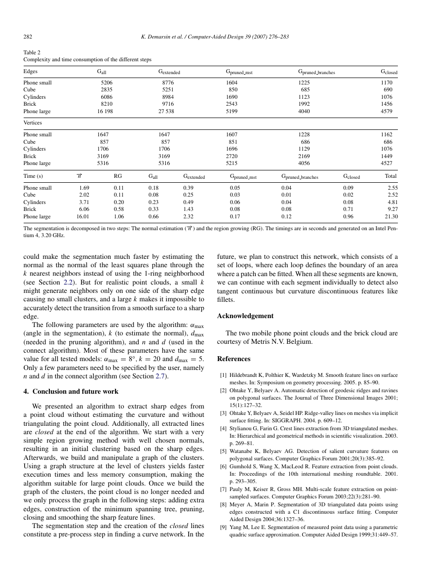In the case of the cube and the cylinders, we see that the segmentation results in the correct number of large clusters: the large clusters ﬁt the extracted sharp feature lines perfectly. Table 2 gives for every step of the algorithm the number of vertices and edges of the corresponding graph. In the case of the two intersecting cylinders, we start with a point cloud of 26 846 points and then we build a graph Gall of 1706 vertices and 6086 edges. After adding edges to Gall, every following step reduces the memory consumption of the graph: a huge reduction in the number of edges happens when building Gpruned mst and Gpruned branches. In general, in the close step, more edges are removed than added, since noisy branches are pruned. Note that for the large mobile phone point cloud the boundary is included just before the close step. The table also illustrates the time consumption of the algorithm. The segmentation step (−→n + RG) requires more time compared to the other steps of the algorithm, because this step has to grow through all the points of the point cloud and the normal for each point needs to be estimated. We

K. Demarsin et al. / Computer-Aided Design 39 (2007) 276–283 281 Fig. 7. Result of each step of the algorithm applied to the cube. (a) Gall; (b) Gextended; (c) Gpruned mst; (d) Gpruned branches; (e) Gclosed; (f) Gsmooth. Fig. 8. Result of each step of the algorithm applied to the mobile phone point cloud. (a) Gall; (b) Gextended; (c) Gpruned mst; (d) Gpruned branches; (e) Gclosed; (f) Gsmooth. Fig. 9. Results for a larger detail of the mobile phone. (a) and (b) illustrate two different views of the segmentation; (c) Gsmooth. Fig. 10. Results for the brick point cloud. (a) Point cloud with ﬂat shading; (b) segmentation; (c) Gpruned branches; (d) Gsmooth.

282 K. Demarsin et al. / Computer-Aided Design 39 (2007) 276–283 Table 2 Complexity and time consumption of the different steps Gextended 8776 5251 8984 9716 27 538 1647 857 1706 3169 5316 Gpruned mst 1604 850 1690 2543 5199 1607 851 1696 2720 5215 Gpruned branches 1225 685 1123 1992 4040 1228 686 1129 2169 4056 Gclosed 1170 690 1076 1456 4579 1162 686 1076 1449 4527 Total Edges Phone small Cube Cylinders Brick Phone large Vertices Phone small Cube Cylinders Brick Phone large Time (s) Gall 5206 2835 6086 8210 16 198 1647 857 1706 3169 5316 RG −→n 1.69 2.02 3.71 6.06 16.01 Phone small 2.55 Cube 2.52 Cylinders 4.81 Brick 9.27 Phone large 21.30 The segmentation is decomposed in two steps: The normal estimation (−→n ) and the region growing (RG). The timings are in seconds and generated on an Intel Pen- tium 4, 3.20 GHz. 0.11 0.11 0.20 0.58 1.06 Gpruned branches 0.04 0.01 0.04 0.08 0.12 Gclosed 0.09 0.02 0.08 0.71 0.96 Gall 0.18 0.08 0.23 0.33 0.66 Gextended 0.39 0.25 0.49 1.43 2.32 Gpruned mst 0.05 0.03 0.06 0.08 0.17 could make the segmentation much faster by estimating the normal as the normal of the least squares plane through the k nearest neighbors instead of using the 1-ring neighborhood (see Section 2.2). But for realistic point clouds, a small k might generate neighbors only on one side of the sharp edge causing no small clusters, and a large k makes it impossible to accurately detect the transition from a smooth surface to a sharp edge. The following parameters are used by the algorithm: αmax (angle in the segmentation), k (to estimate the normal), dmax (needed in the pruning algorithm), and n and d (used in the connect algorithm). Most of these parameters have the same value for all tested models: αmax = 8◦, k = 20 and dmax = 5. Only a few parameters need to be speciﬁed by the user, namely n and d in the connect algorithm (see Section 2.7). 4. Conclusion and future work We presented an algorithm to extract sharp edges from a point cloud without estimating the curvature and without triangulating the point cloud. Additionally, all extracted lines are closed at the end of the algorithm. We start with a very simple region growing method with well chosen normals, resulting in an initial clustering based on the sharp edges. Afterwards, we build and manipulate a graph of the clusters. Using a graph structure at the level of clusters yields faster execution times and less memory consumption, making the algorithm suitable for large point clouds. Once we build the graph of the clusters, the point cloud is no longer needed and we only process the graph in the following steps: adding extra edges, construction of the minimum spanning tree, pruning, closing and smoothing the sharp feature lines. The segmentation step and the creation of the closed lines constitute a pre-process step in ﬁnding a curve network. In the future, we plan to construct this network, which consists of a set of loops, where each loop deﬁnes the boundary of an area where a patch can be ﬁtted. When all these segments are known, we can continue with each segment individually to detect also tangent continuous but curvature discontinuous features like ﬁllets. Acknowledgement The two mobile phone point clouds and the brick cloud are courtesy of Metris N.V. Belgium. References [1] Hildebrandt K, Polthier K, Wardetzky M. Smooth feature lines on surface meshes. In: Symposium on geometry processing. 2005. p. 85–90. [2] Ohtake Y, Belyaev A. Automatic detection of geodesic ridges and ravines on polygonal surfaces. The Journal of Three Dimensional Images 2001; 15(1):127–32. [3] Ohtake Y, Belyaev A, Seidel HP. Ridge-valley lines on meshes via implicit surface ﬁtting. In: SIGGRAPH. 2004. p. 609–12. [4] Stylianou G, Farin G. Crest lines extraction from 3D triangulated meshes. In: Hierarchical and geometrical methods in scientiﬁc visualization. 2003. p. 269–81. [5] Watanabe K, Belyaev AG. Detection of salient curvature features on polygonal surfaces. Computer Graphics Forum 2001;20(3):385–92. [6] Gumhold S, Wang X, MacLeod R. Feature extraction from point clouds. In: Proceedings of the 10th international meshing roundtable. 2001. p. 293–305. [7] Pauly M, Keiser R, Gross MH. Multi-scale feature extraction on point- sampled surfaces. Computer Graphics Forum 2003;22(3):281–90. [8] Meyer A, Marin P. Segmentation of 3D triangulated data points using edges constructed with a C1 discontinuous surface ﬁtting. Computer Aided Design 2004;36:1327–36. [9] Yang M, Lee E. Segmentation of measured point data using a parametric quadric surface approximation. Computer Aided Design 1999;31:449–57.

K. Demarsin et al. / Computer-Aided Design 39 (2007) 276–283 283 [10] Vanco M, Brunnett G, Schreiber Th. A direct approach towards automatic surface segmentation of unorganized 3d points. In: Proceedings spring conference on computer graphics. 2000. p. 185–94. [11] Vanco M, Brunnett G. Direct segmentation for reverse engineering. In: Proceedings international symposium on cyber worlds. 2002. p. 24–37. [12] Vanco M, Brunnett G. Direct segmentation of algebraic models for reverse engineering. Computing 2004;72(1–2):207–20. [13] Demarsin K, Vanderstraeten D, Volodine T, Roose D. Detection of closed sharp feature lines in point clouds for reverse engineering applications. In: Proceedings of geometric modeling and processing. 2006. p. 571–7. [14] Floater MS, Reimers M. Meshless parameterization and surface reconstruction. Computer Aided Geometric Design 2001;18(2):77–92. [15] Hormann K. Theory and applications of parameterizing triangulations. Ph.D. thesis. Department of computer science, University of Erlangen; 2001. [16] Volodine T, Vanderstraeten D, Roose D. Smoothing of meshes and point clouds using weighted geometry-aware bases. Report TW 451. Belgium: Department of computer science, K.U. Leuven; 2006.

分享到：

赞收藏

资料库

点云分割基于特征边界提取.pdf

相关推荐

行业

热门标签

最新资料