Pattern Recognition 43 (2010) 255 -- 266
Contents lists available at ScienceDirect
Pattern Recognition
journal homepage: w w w . e l s e v i e r . c o m / l o c a t e / p r
Topological active volumes: A topology-adaptive deformable model for
volume segmentation
N. Barreira a,∗, M.G. Penedo a, L. Cohen b, M. Ortega a
aUniversity of A Coruña, Department of Computer Science, A Coruña, Spain
bCEREMADE, Universite Paris Dauphine, France
A R T I C L E
I N F O
A B S T R A C T
Article history:
Received 9 February 2009
Received in revised form 22 May 2009
Accepted 11 June 2009
Keywords:
3D image segmentation
Topological active volumes
Adaptive topology
This paper proposes a generic methodology for segmentation and reconstruction of volumetric datasets
based on a deformable model, the topological active volumes (TAV). This model, based on a polyhedral
mesh, integrates features of region-based and boundary-based segmentation methods in order to fit the
contours of the objects and model its inner topology. Moreover, it implements automatic procedures,
the so-called topological changes, that alter the mesh structure and allow the segmentation of complex
features such as pronounced curvatures or holes, as well as the detection of several objects in the scene.
This work presents the TAV model and the segmentation methodology and explains how the changes
in the TAV structure can improve the adjustment process. In particular, it is focused on the increase of
the mesh density in complex image areas in order to improve the adjustment to object surfaces. The
suitability of the mesh structure and the segmentation methodology is analyzed and the accuracy of the
proposed model is proved with both synthetic and real images.
© 2009 Elsevier Ltd. All rights reserved.
1. Introduction
The recent development of 3D acquisition technologies has
emphasized the need of techniques for the understanding of vol-
umetric datasets in several fields such as medical imaging [1,2] or
non-destructive testing of products [3,4]. Object segmentation and
reconstruction are important tasks in the image processing pipeline.
Nevertheless, the detection of objects in volumetric datasets is a
challenging problem due to the size of the data and the variability
of the features of interest.
Deformable models are well-known tools in image analysis
that have been applied successfully in several fields such as image
segmentation and reconstruction, pattern recognition, surgery sim-
ulation or tracking. They were introduced by Kass et al. [5] and
generalized to 3D by Terzopoulos et al. [6].
Deformable models can be broadly classified into explicit or im-
plicit models. On one hand, the explicit techniques represent the
object by means of meshes (curves, surfaces or solids) which shape
evolves under the influence of external and internal forces. The shape
deformation is the main advantage of this kind of models since it
∗ Corresponding author. Fax: +34 981 167 160.
E-mail addresses: nbarreira@udc.es (N. Barreira), mgpenedo@udc.es
(M.G. Penedo), cohen@ceremade.dauphine.fr (L. Cohen), mortega@udc.es (M. Ortega).
0031-3203/$ - see front matter © 2009 Elsevier Ltd. All rights reserved.
doi:10.1016/j.patcog.2009.06.005
allows the adjustment to different objects. However, since the model
topology is created before the deformations, deformable models
are not generally able to segment complex shapes with genus
higher than 0. In order to overcome this limitation, several works
have been developed in past years. McInerney and Terzopoulos [7]
have proposed the T-snakes, an extension of the classic snakes that
enables topological flexibility by means of an iterative reparametriza-
tion of the contours. To this end, they decompose the image domain
into a discrete grid and compute the intersections between the
contour and the grid. Delingette and Montagnat [8], Duan and Qin
[9] and Lachaud et al. [10,11] have developed techniques based on
detecting the self-intersections in the evolving mesh and merging
the colliding regions using a set of remeshing rules. Moreover, Pons
and Boissonat [12] have proposed an approach where the mesh is
iteratively updated by computing the restricted Delaunay triangu-
lation of the deformed objects. On the other hand, the geometric
deformable models [13,14] are based on the level set formulation
[15] and they are represented implicitly. This kind of representa-
tion of contours and surfaces provides topological flexibility in the
segmentation process so that the topological changes are automati-
cally handled. However, it makes difficult the user interaction and
increases the computational cost. Nevertheless, some optimizations
have been proposed to increase the efficiency of the segmentation
process [16,17].
The topological active volume (TAV) [18] is a parametric 3D
deformable model based on the active nets model. The active nets
�
256
N. Barreira et al. / Pattern Recognition 43 (2010) 255 -- 266
model was first proposed by Tsumiyama and Yamamoto [19] as a
variant of the deformable models that integrates features of region-
based and boundary-based segmentation techniques. To this end,
this model has two different kinds of nodes: external nodes for sur-
face adjustment and internal nodes for modelling the inner topology.
The former uses boundary information whereas the latter is related
to the region information. This duality is the main advantage of this
model over other models as level sets since it allows not only the
surface adjustment but also the analysis of the inner object features.
The nodes are organized in a polyhedral mesh that is deformed un-
der the influence of energy functions.
Besides, another advantage of the TAV model is its ability to
perform topological changes in its structure in order to adjust to
concavities, detect holes and find separate objects in the scene. The
topological adaptation in the TAV model is based on the detection
of complex areas in the scene and the development of appropriate
changes in the mesh topology to achieve the adjustment. The com-
plex areas are detected by means of computing several variables re-
lated to the mesh features whereas the changes are related to the
insertion, deletion or transformation of nodes. This way, the inser-
tion of new nodes in areas with pronounced curvatures improves
the mesh adjustment. Also, the deletion of nodes allows the adjust-
ment to convex areas as well as the detection of several objects in
the scene. Finally, the transformation of the type of node is used for
detecting features such as holes inside the objects.
This paper reviews the model and segmentation methodology as
well as describes the techniques to modify the TAV structure based
on the removal of nodes in order to improve the segmentation re-
sults. In this sense, this paper is focused on the analysis of complex
image areas using the structure tensor in order to detect object cur-
vatures. The increase of the mesh density in these areas improves
the adjustment to the object surfaces. To this end, this paper pro-
poses several procedures to add new nodes to the existing mesh.
Moreover, the features of the mesh topology as well as the proposed
methodology are analyzed and compared with other techniques. Fi-
nally, several segmentation results on images with different com-
plexity are presented.
This paper is organized as follows. Section 2 presents the fea-
tures of the TAV model. Section 3 explains the steps followed in the
segmentation process. Section 4 reviews how the TAV model can
perform topological changes in order to detect complex structures
in the scene. Section 5 shows some segmentation results that prove
the model suitability and finally Section 6 presents the conclusions
and the intended future work.
2. Model
A topological active volume is a three-dimensional structure com-
posed of interrelated nodes located at the vertices of a polyhedron
[18]. This polyhedron is repeated throughout the mesh and defines
the neighboring relationships among nodes. There are two types of
nodes: internal, inside the mesh, and external, on the surfaces. Each
type of node represents different object features. The external nodes
fit the surface of the object whereas the internal nodes model its in-
ner topology. This fact allows the integration of information based
on discontinuities and information based on regions. The former is
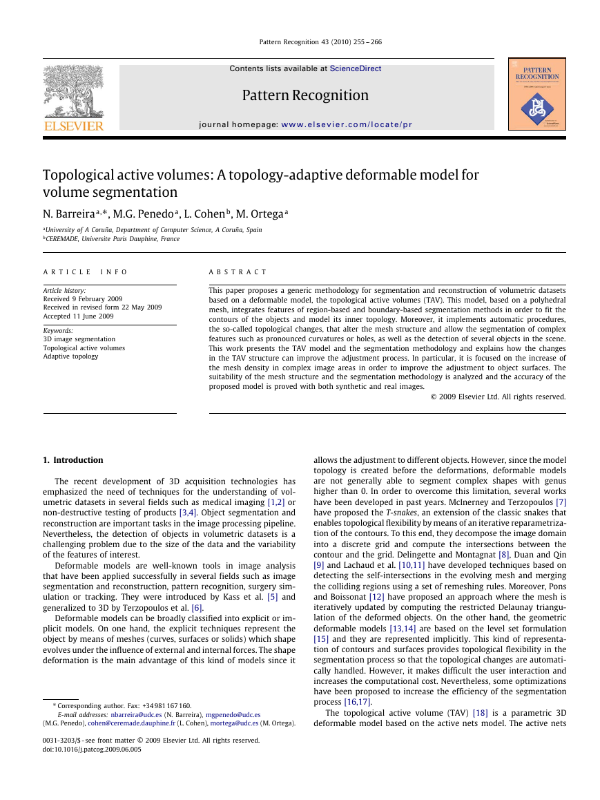
associated to external nodes and the latter to internal nodes. Fig. 1
shows TAVs with cubic and tetrahedral topologies.
Parametrically, a TAV is defined as v(r, s, t) = (x(r, s, t), y(r, s, t),
z(r, s, t)), where (r, s, t) ∈ ([0, 1]×[0, 1]×[0, 1]). The state of the model
is governed by an energy function defined as follows:
1
1
1
Eint(v(r, s, t)) + Eext(v(r, s, t)) dr ds dt
E(v) =
(1)
0
0
0
Fig. 1. TAV meshes with 3×3×3 nodes. The dark nodes represent the external nodes
whereas the light one is the internal node. Left: cubic mesh; right: tetrahedral mesh.
where Eint and Eext are the internal and the external energy of the
TAV, respectively. The former controls the shape and the structure
of the net. Its calculus depends on first and second order derivatives
which control contraction and bending, respectively. The internal
energy term is defined by
Eint(v(r, s, t)) = ♡(|vr(r, s, t)|2 + |vs(r, s, t)|2 + |vt(r, s, t)|2)
+ ♢(|vrr(r, s, t)|2 + |vss(r, s, t)|2 + |vtt(r, s, t)|2)
+ 2♤(|vrs(r, s, t)|2 + |vrt(r, s, t)|2 + |vst(r, s, t)|2)
(2)
where subscripts represent partial derivatives and ♡, ♢ and ♤ are co-
efficients that control the smoothness of the net. In order to compute
the energy, the parameter domain [0, 1]× [0, 1]× [0, 1] is discretized
as a regular grid defined by the internode spacing (k, l, m) and the
first and second derivatives are estimated using the finite differences
technique in 3D.
Eext represents the features of the scene that guide the adjustment
process and is defined as follows:
Eext(v(r, s, t)) = ♽f [I(v(r, s, t))] +
♵
|ℵ(r, s, t)|
1
×
p∈ℵ(r,s,t)
||v(r, s, t) − v(p)|| f [I(v(p))]
(3)
where ♽ and ♵ are weights, I(v(r, s, t)) is the intensity value of the
original image in the position v(r, s, t), f is a function related to the
image intensity, and ℵ(r, s, t) is the neighborhood of the node (r, s, t).
This way, given that the repeated polyhedron in the mesh defines
the node neighborhoods, the shape of the polyhedron influences
not only the flexibility of the mesh, but also the way the nodes are
adjusted to the objects.
Since the internal and external nodes model different parts of the
objects, f should be adapted for both types of nodes. On one hand, if
the objects to detect are dark and the background is light, the energy
of an internal node will be minimum when it is on a point with a
low gray level. On the other hand, the energy of an external node
will be minimum when it is on a discontinuity and on a light point
outside the object. In this situation, function f is defined as
⎧⎨
⎩h[I(v)n]
for internal nodes
h[Imax − I(v)n
+♱(Gmax − G(v))] + GD(v)
f [I(v)] =
for external nodes
(4)
where ♱ is a weighting term, Imax and Gmax are the maximum in-
tensity values of image I and the gradient image G, respectively, I(v)
and G(v) are the intensity values of the original image and the gra-
dient image in the node position v(r, s, t), I(v)n is the mean intensity
in a n × n × n cube, h is an appropriate scaling function, and GD(v)
is the gradient distance, that is, the distance from the node position
v(r, s, t) to its nearest edge. This way, the combination of gradient
terms and intensity values in an area allows the integration of both
boundary and region information in the external energy term.
�
N. Barreira et al. / Pattern Recognition 43 (2010) 255 -- 266
257
3. Segmentation methodology
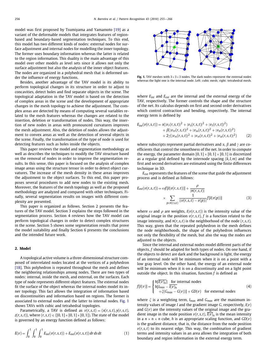
The segmentation process consists of several stages as Fig. 2
shows. First, a mesh with a homogeneous distribution of nodes is
created and located automatically over the whole image. This way,
the mesh is able to detect objects located throughout the scene. After
the initialization stage, the mesh energy is minimized iteratively by
means of a greedy algorithm. This algorithm iteratively moves the
mesh nodes to neighboring voxels where the node energy is lower.
It stops when the energy functions reach a minimum, that is, when
the mesh is located around the objects.
After the minimization stage, the number of nodes in each axis is
recomputed to adapt the mesh size to the object size; for example,
if the object is longer than wider, the number of nodes in the x-axis
will be increased whereas the number of nodes in the y-axis will be
decreased. The mesh is also centered over the detected objects in
order to get a node distribution independent of the object location.
Then, the mesh energy is minimized again.
Finally, topological changes are performed to increase the flex-
ibility of the model and, after a local energy minimization step, to
adjust the mesh to concave surfaces, holes, or separate objects. There
are three kinds of topological changes. First, the removal of nodes al-
lows the adjustment to concave surfaces and the detection of several
objects in the scene. Second, special features such as internal holes
can be detected by changing the behavior of some nodes. Finally, the
insertion of new nodes increases the accuracy of the adjustment to
corners and sharp edges.
The TAV model has been developed using several base polyhe-
dra. A topology based on cubes was implemented first. Even though
the segmentation results using this configuration were good [18],
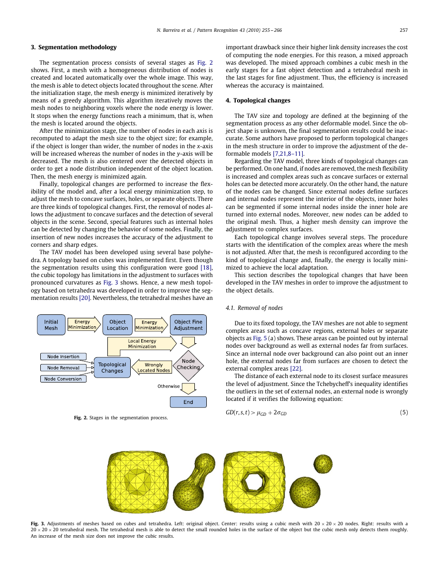
the cubic topology has limitations in the adjustment to surfaces with
pronounced curvatures as Fig. 3 shows. Hence, a new mesh topol-
ogy based on tetrahedra was developed in order to improve the seg-
mentation results [20]. Nevertheless, the tetrahedral meshes have an
Fig. 2. Stages in the segmentation process.
important drawback since their higher link density increases the cost
of computing the node energies. For this reason, a mixed approach
was developed. The mixed approach combines a cubic mesh in the
early stages for a fast object detection and a tetrahedral mesh in
the last stages for fine adjustment. Thus, the efficiency is increased
whereas the accuracy is maintained.
4. Topological changes
The TAV size and topology are defined at the beginning of the
segmentation process as any other deformable model. Since the ob-
ject shape is unknown, the final segmentation results could be inac-
curate. Some authors have proposed to perform topological changes
in the mesh structure in order to improve the adjustment of the de-
formable models [7,21,8–11].
Regarding the TAV model, three kinds of topological changes can
be performed. On one hand, if nodes are removed, the mesh flexibility
is increased and complex areas such as concave surfaces or external
holes can be detected more accurately. On the other hand, the nature
of the nodes can be changed. Since external nodes define surfaces
and internal nodes represent the interior of the objects, inner holes
can be segmented if some internal nodes inside the inner hole are
turned into external nodes. Moreover, new nodes can be added to
the original mesh. Thus, a higher mesh density can improve the
adjustment to complex surfaces.
Each topological change involves several steps. The procedure
starts with the identification of the complex areas where the mesh
is not adjusted. After that, the mesh is reconfigured according to the
kind of topological change and, finally, the energy is locally mini-
mized to achieve the local adaptation.
This section describes the topological changes that have been
developed in the TAV meshes in order to improve the adjustment to
the object details.
4.1. Removal of nodes
Due to its fixed topology, the TAV meshes are not able to segment
complex areas such as concave regions, external holes or separate
objects as Fig. 5 (a) shows. These areas can be pointed out by internal
nodes over background as well as external nodes far from surfaces.
Since an internal node over background can also point out an inner
hole, the external nodes far from surfaces are chosen to detect the
external complex areas [22].
The distance of each external node to its closest surface measures
the level of adjustment. Since the Tchebycheff's inequality identifies
the outliers in the set of external nodes, an external node is wrongly
located if it verifies the following equation:
GD(r, s, t) > ♯GD + 2♶GD
(5)
Fig. 3. Adjustments of meshes based on cubes and tetrahedra. Left: original object. Center: results using a cubic mesh with 20 × 20 × 20 nodes. Right: results with a
20 × 20 × 20 tetrahedral mesh. The tetrahedral mesh is able to detect the small rounded holes in the surface of the object but the cubic mesh only detects them roughly.
An increase of the mesh size does not improve the cubic results.
�
258
N. Barreira et al. / Pattern Recognition 43 (2010) 255 -- 266
where GD(r, s, t) stands for the gradient distance of the external node
(r, s, t), and ♯GD and ♶GD are the average and standard deviation of
the gradient distances of the set of external nodes, respectively. We
are considering that the 25% of the external nodes can be outliers.
In the node removal procedure, there is a priority that weights
the gradient distance. This priority forces the removal of nodes in
the same area in order to avoid anarchical removals that sometimes
cause a wrong segmentation result. At the beginning, the priority of
each node is initialized to 1 and this value is doubled every time that
a topological change is performed in the neighborhood of a node.
Once the set of external nodes far away from the object bound-
aries is identified, next node to remove is the node that fulfils
GD(r, s, t) ∗ p(r, s, t) > GD(r
(r
, t
),
) ∈ {(x, y, z)|GD(x, y, z) > ♯GD + 2♶GD}
, s
, s
) ∗ p(r
, s
, t
, t
(6)
where p(r, s, t) is the priority of the node (r, s, t). Thus, the choice of
a node to remove relies on the node location in the image and on
earlier node removals in the node neighborhood.
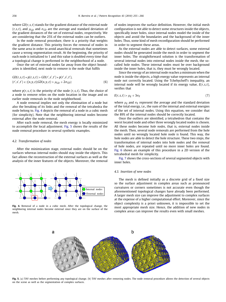
A node removal implies not only the elimination of a node but
also the breaking of its links and the removal of the tetrahedra the
node belong to. Fig. 4 depicts the removal of a node in a cubic mesh
(for simplicity). Note that the neighboring internal nodes become
external after the node removal.
After each node removal, the mesh energy is locally minimized
to accomplish the local adjustment. Fig. 5 shows the results of the
node removal procedure in several synthetic examples.
4.2. Transformation of nodes
After the minimization stage, external nodes should be on the
surfaces whereas internal nodes should stay inside the objects. This
fact allows the reconstruction of the external surfaces as well as the
analysis of the inner features of the objects. Moreover, the removal
Internal nodes
External nodes
Fig. 4. Removal of a node in a cubic mesh. After the topological change, the
neighboring internal nodes become external since they are on the surface of the
mesh.
of nodes improves the surface definition. However, the initial mesh
configuration is not able to detect some structures inside the objects,
specifically inner holes, since internal nodes model the inside of the
objects and avoid the boundaries and the background of the inner
holes. Thus, some kind of mesh reconfiguration should be performed
in order to segment these areas.
As the external nodes are able to detect surfaces, some external
nodes should be generated inside the mesh in order to segment the
inner holes. The straightforward solution is the transformation of
several internal nodes into external nodes inside the mesh, the so-
called hole nodes. These internal nodes must be over background
inside the inner holes, that is, they must be wrongly located.
Since the energy of an internal node reaches a minimum when the
node is inside the objects, a high energy value represents an internal
node not correctly located. Using the Tchebycheff's inequality, an
internal node will be wrongly located if its energy value, E(r, s, t),
verifies that
E(r, s, t) > ♯E + 3♶E
(7)
where ♯E and ♶E represent the average and the standard deviation
of the total energy, i.e., the sum of the internal and external energies
of the set of internal nodes. Using this equation, we consider that
the 89% of the internal nodes should be correctly located.
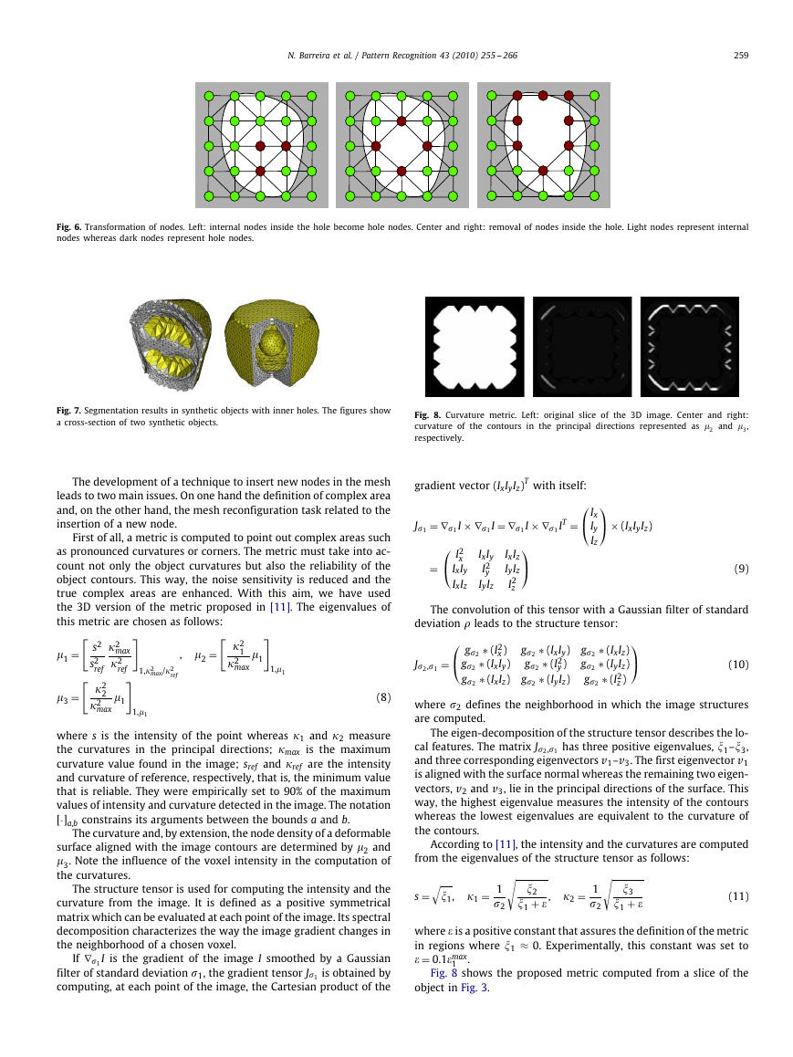
Once the outliers are identified, a tetrahedron that contains the
worst located node and other three wrongly located nodes is chosen.
All these nodes become hole nodes, that is, external nodes inside
the mesh. Then, several node removals are performed from the hole
nodes until no wrongly located hole node is found. This way, the
hole nodes are able to detect the hole structure. These two steps, the
transformation of internal nodes into hole nodes and the removal
of hole nodes, are repeated until no more inner holes are found.
Fig. 6 shows an example of this procedure in a 2D version of the
tetrahedral mesh for simplicity.
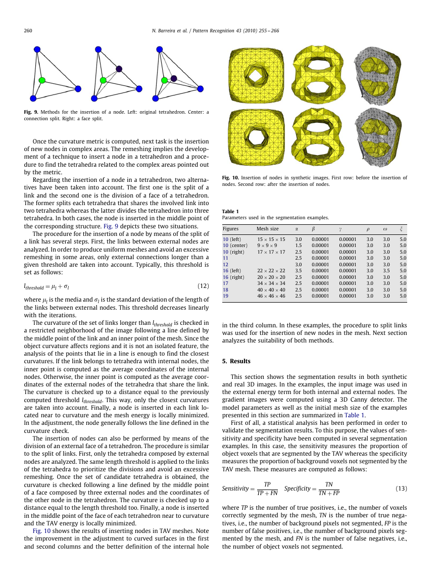
Fig. 7 shows the cross-sections of several segmented objects with
inner holes.
4.3. Insertion of new nodes
The mesh is defined initially as a discrete grid of a fixed size
so the surface adjustment in complex areas such as pronounced
curvatures or corners sometimes is not accurate even though the
aforementioned topological changes have already been performed.
A larger mesh size can improve the adjustment to complex surfaces
at the expense of a higher computational effort. Moreover, since the
object complexity is a priori unknown, it is impossible to set the
most appropriate mesh size. Hence, the addition of new nodes in
complex areas can improve the results even with small meshes.
Fig. 5. (a) TAV meshes before performing any topological change. (b) TAV meshes after removing nodes. The node removal procedure allows the detection of several objects
on the scene as well as the segmentation of complex surfaces.
�
N. Barreira et al. / Pattern Recognition 43 (2010) 255 -- 266
259
Fig. 6. Transformation of nodes. Left: internal nodes inside the hole become hole nodes. Center and right: removal of nodes inside the hole. Light nodes represent internal
nodes whereas dark nodes represent hole nodes.
Fig. 7. Segmentation results in synthetic objects with inner holes. The figures show
a cross-section of two synthetic objects.
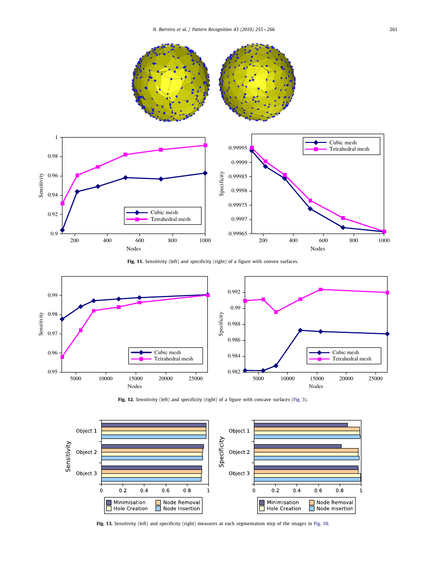
Fig. 8. Curvature metric. Left: original slice of the 3D image. Center and right:
curvature of the contours in the principal directions represented as ♯
2 and ♯
3,
respectively.
The development of a technique to insert new nodes in the mesh
leads to two main issues. On one hand the definition of complex area
and, on the other hand, the mesh reconfiguration task related to the
insertion of a new node.
First of all, a metric is computed to point out complex areas such
as pronounced curvatures or corners. The metric must take into ac-
count not only the object curvatures but also the reliability of the
object contours. This way, the noise sensitivity is reduced and the
true complex areas are enhanced. With this aim, we have used
the 3D version of the metric proposed in [11]. The eigenvalues of
this metric are chosen as follows:
gradient vector (IxIyIz)T with itself:
⎛
⎝ Ix
= ∇♶1 I × ∇♶1 I = ∇♶1 I × ∇♶1 IT =
⎛
⎝ I2
⎞
⎠
Iy
Iz
J♶1
=
x
IxIy
IxIz
IxIy
I2
y
IyIz
IxIz
IyIz
I2
z
⎞
⎠ × (IxIyIz)
(9)
The convolution of this tensor with a Gaussian filter of standard
deviation ♵ leads to the structure tensor:
1,♯1
=
J♶2,♶1
(10)
, ♯2 =
1,♭2
max/♭2
ref
♭2
1
♭2
max
♯1
♯1 =
♯3 =
♭2
max
♭2
ref
s2
s2
ref
♭2
2
♭2
max
♯1
1,♯1
(8)
where s is the intensity of the point whereas ♭1 and ♭2 measure
the curvatures in the principal directions; ♭max is the maximum
curvature value found in the image; sref and ♭ref are the intensity
and curvature of reference, respectively, that is, the minimum value
that is reliable. They were empirically set to 90% of the maximum
values of intensity and curvature detected in the image. The notation
[·]a,b constrains its arguments between the bounds a and b.
The curvature and, by extension, the node density of a deformable
surface aligned with the image contours are determined by ♯2 and
♯3. Note the influence of the voxel intensity in the computation of
the curvatures.
The structure tensor is used for computing the intensity and the
curvature from the image. It is defined as a positive symmetrical
matrix which can be evaluated at each point of the image. Its spectral
decomposition characterizes the way the image gradient changes in
the neighborhood of a chosen voxel.
If ∇♶1 I is the gradient of the image I smoothed by a Gaussian
filter of standard deviation ♶1, the gradient tensor J♶1 is obtained by
computing, at each point of the image, the Cartesian product of the
⎛
⎝ g♶2
g♶2
g♶2
∗ (I2
x )
∗ (IxIy)
∗ (IxIz)
∗ (IxIy) g♶2
∗ (I2
y)
g♶2
∗ (IyIz)
g♶2
∗ (IxIz)
∗ (IyIz)
∗ (I2
z )
g♶2
g♶2
g♶2
⎞
⎠
where ♶2 defines the neighborhood in which the image structures
are computed.
The eigen-decomposition of the structure tensor describes the lo-
cal features. The matrix J♶2,♶1 has three positive eigenvalues, ♱1–♱3,
and three corresponding eigenvectors v1–v3. The first eigenvector v1
is aligned with the surface normal whereas the remaining two eigen-
vectors, v2 and v3, lie in the principal directions of the surface. This
way, the highest eigenvalue measures the intensity of the contours
whereas the lowest eigenvalues are equivalent to the curvature of
the contours.
According to [11], the intensity and the curvatures are computed
from the eigenvalues of the structure tensor as follows:
s =
♱1, ♭1 = 1
♶2
♱2
♱1 + ♦ , ♭2 = 1
♶2
♱3
♱1 + ♦
(11)
where ♦ is a positive constant that assures the definition of the metric
in regions where ♱1 ≈ 0. Experimentally, this constant was set to
♦ = 0.1♦max
.
Fig. 8 shows the proposed metric computed from a slice of the
1
object in Fig. 3.
�
260
N. Barreira et al. / Pattern Recognition 43 (2010) 255 -- 266
Fig. 9. Methods for the insertion of a node. Left: original tetrahedron. Center: a
connection split. Right: a face split.
Once the curvature metric is computed, next task is the insertion
of new nodes in complex areas. The remeshing implies the develop-
ment of a technique to insert a node in a tetrahedron and a proce-
dure to find the tetrahedra related to the complex areas pointed out
by the metric.
Regarding the insertion of a node in a tetrahedron, two alterna-
tives have been taken into account. The first one is the split of a
link and the second one is the division of a face of a tetrahedron.
The former splits each tetrahedra that shares the involved link into
two tetrahedra whereas the latter divides the tetrahedron into three
tetrahedra. In both cases, the node is inserted in the middle point of
the corresponding structure. Fig. 9 depicts these two situations.
The procedure for the insertion of a node by means of the split of
a link has several steps. First, the links between external nodes are
analyzed. In order to produce uniform meshes and avoid an excessive
remeshing in some areas, only external connections longer than a
given threshold are taken into account. Typically, this threshold is
set as follows:
lthreshold = ♯l + ♶l
(12)
where ♯l is the media and ♶l is the standard deviation of the length of
the links between external nodes. This threshold decreases linearly
with the iterations.
The curvature of the set of links longer than lthreshold is checked in
a restricted neighborhood of the image following a line defined by
the middle point of the link and an inner point of the mesh. Since the
object curvature affects regions and it is not an isolated feature, the
analysis of the points that lie in a line is enough to find the closest
curvatures. If the link belongs to tetrahedra with internal nodes, the
inner point is computed as the average coordinates of the internal
nodes. Otherwise, the inner point is computed as the average coor-
dinates of the external nodes of the tetrahedra that share the link.
The curvature is checked up to a distance equal to the previously
computed threshold lthreshold. This way, only the closest curvatures
are taken into account. Finally, a node is inserted in each link lo-
cated near to curvature and the mesh energy is locally minimized.
In the adjustment, the node generally follows the line defined in the
curvature check.
The insertion of nodes can also be performed by means of the
division of an external face of a tetrahedron. The procedure is similar
to the split of links. First, only the tetrahedra composed by external
nodes are analyzed. The same length threshold is applied to the links
of the tetrahedra to prioritize the divisions and avoid an excessive
remeshing. Once the set of candidate tetrahedra is obtained, the
curvature is checked following a line defined by the middle point
of a face composed by three external nodes and the coordinates of
the other node in the tetrahedron. The curvature is checked up to a
distance equal to the length threshold too. Finally, a node is inserted
in the middle point of the face of each tetrahedron near to curvature
and the TAV energy is locally minimized.
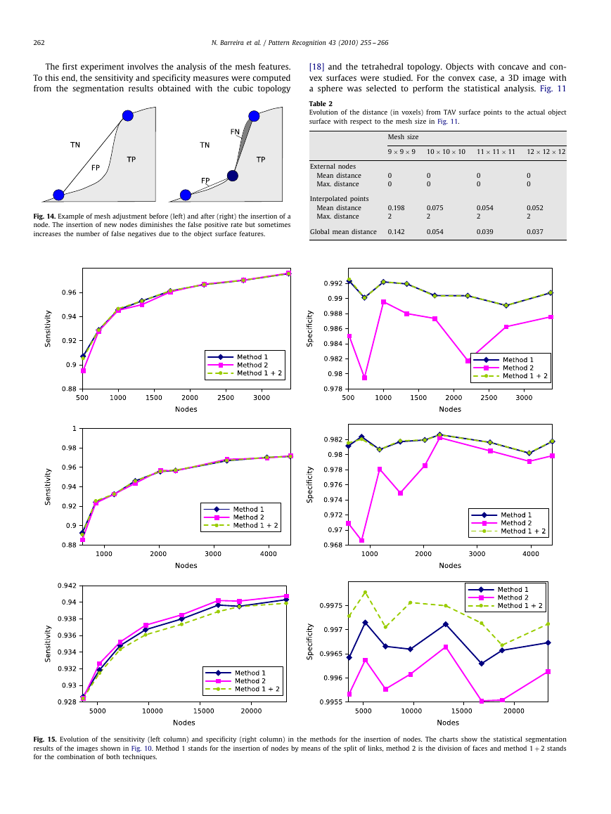
Fig. 10 shows the results of inserting nodes in TAV meshes. Note
the improvement in the adjustment to curved surfaces in the first
and second columns and the better definition of the internal hole
Fig. 10. Insertion of nodes in synthetic images. First row: before the insertion of
nodes. Second row: after the insertion of nodes.
Table 1
Parameters used in the segmentation examples.
Figures
10 (left)
10 (center)
10 (right)
11
12
16 (left)
16 (right)
17
18
19
Mesh size
15 × 15 × 15
9 × 9 × 9
17 × 17 × 17
22 × 22 × 22
20 × 20 × 20
34 × 34 × 34
40 × 40 × 40
46 × 46 × 46
♡
3.0
1.5
2.5
2.5
3.0
3.5
2.5
2.5
2.5
2.5
♢
♤
0.00001
0.00001
0.00001
0.00001
0.00001
0.00001
0.00001
0.00001
0.00001
0.00001
0.00001
0.00001
0.00001
0.00001
0.00001
0.00001
0.00001
0.00001
0.00001
0.00001
♵
3.0
3.0
3.0
3.0
3.0
3.0
3.0
3.0
3.0
3.0
♽
3.0
3.0
3.0
3.0
3.0
3.5
3.0
3.0
3.0
3.0
♱
5.0
5.0
5.0
5.0
5.0
5.0
5.0
5.0
5.0
5.0
in the third column. In these examples, the procedure to split links
was used for the insertion of new nodes in the mesh. Next section
analyzes the suitability of both methods.
5. Results
This section shows the segmentation results in both synthetic
and real 3D images. In the examples, the input image was used in
the external energy term for both internal and external nodes. The
gradient images were computed using a 3D Canny detector. The
model parameters as well as the initial mesh size of the examples
presented in this section are summarized in Table 1.
First of all, a statistical analysis has been performed in order to
validate the segmentation results. To this purpose, the values of sen-
sitivity and specificity have been computed in several segmentation
examples. In this case, the sensitivity measures the proportion of
object voxels that are segmented by the TAV whereas the specificity
measures the proportion of background voxels not segmented by the
TAV mesh. These measures are computed as follows:
Sensitivity =
TP
TP + FN
Specificity = TN
TN + FP
(13)
where TP is the number of true positives, i.e., the number of voxels
correctly segmented by the mesh, TN is the number of true nega-
tives, i.e., the number of background pixels not segmented, FP is the
number of false positives, i.e., the number of background pixels seg-
mented by the mesh, and FN is the number of false negatives, i.e.,
the number of object voxels not segmented.
�
N. Barreira et al. / Pattern Recognition 43 (2010) 255 -- 266
261
y
t
i
v
i
t
i
s
n
e
S
1
0.98
0.96
0.94
0.92
0.9
0.99
y
t
i
v
i
t
i
s
n
e
S
0.98
0.97
0.96
0.95
Cubic mesh
Tetrahedral mesh
y
t
i
c
i
f
i
c
e
p
S
0.99995
0.9999
0.99985
0.9998
0.99975
0.9997
0.99965
Cubic mesh
Tetrahedral mesh
200
400
600
Nodes
800
1000
200
400
600
Nodes
800
1000
Fig. 11. Sensitivity (left) and specificity (right) of a figure with convex surfaces.
y
t
i
c
i
f
i
c
e
p
S
0.992
0.99
0.988
0.986
0.984
0.982
Cubic mesh
Tetrahedral mesh
Cubic mesh
Tetrahedral mesh
5000
10000
15000
Nodes
20000
25000
5000
10000
15000
Nodes
20000
25000
Fig. 12. Sensitivity (left) and specificity (right) of a figure with concave surfaces (Fig. 3).
Fig. 13. Sensitivity (left) and specificity (right) measures at each segmentation step of the images in Fig. 10.
�
262
N. Barreira et al. / Pattern Recognition 43 (2010) 255 -- 266
The first experiment involves the analysis of the mesh features.
To this end, the sensitivity and specificity measures were computed
from the segmentation results obtained with the cubic topology
[18] and the tetrahedral topology. Objects with concave and con-
vex surfaces were studied. For the convex case, a 3D image with
a sphere was selected to perform the statistical analysis. Fig. 11
Table 2
Evolution of the distance (in voxels) from TAV surface points to the actual object
surface with respect to the mesh size in Fig. 11.
Mesh size
9 × 9 × 9
0
0
0.198
2
External nodes
Mean distance
Max. distance
Interpolated points
Mean distance
Max. distance
Global mean distance
0.142
10 × 10 × 10
11 × 11 × 11
12 × 12 × 12
0
0
0.075
2
0.054
0
0
0.054
2
0.039
0
0
0.052
2
0.037
Fig. 14. Example of mesh adjustment before (left) and after (right) the insertion of a
node. The insertion of new nodes diminishes the false positive rate but sometimes
increases the number of false negatives due to the object surface features.
Fig. 15. Evolution of the sensitivity (left column) and specificity (right column) in the methods for the insertion of nodes. The charts show the statistical segmentation
results of the images shown in Fig. 10. Method 1 stands for the insertion of nodes by means of the split of links, method 2 is the division of faces and method 1 + 2 stands
for the combination of both techniques.
�


 2023年江西萍乡中考道德与法治真题及答案.doc
 2012年重庆南川中考生物真题及答案.doc
 2013年江西师范大学地理学综合及文艺理论基础考研真题.doc
 2020年四川甘孜小升初语文真题及答案I卷.doc
 2020年注册岩土工程师专业基础考试真题及答案.doc
 2023-2024学年福建省厦门市九年级上学期数学月考试题及答案.doc
 2021-2022学年辽宁省沈阳市大东区九年级上学期语文期末试题及答案.doc
 2022-2023学年北京东城区初三第一学期物理期末试卷及答案.doc
 2018上半年江西教师资格初中地理学科知识与教学能力真题及答案.doc
 2012年河北国家公务员申论考试真题及答案-省级.doc
 2020-2021学年江苏省扬州市江都区邵樊片九年级上学期数学第一次质量检测试题及答案.doc
 2022下半年黑龙江教师资格证中学综合素质真题及答案.doc